Page 9 - Summer 2008

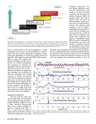
Fig. 1. Signal processing approach: the model-based “staircase.” \[Step 1\] “Simple” non-parametric implicit models. \[Step 2\] “Black-box” models (transfer function, autoregressive, moving average, polynomial, etc.). \[Step 3\] “Gray-box” models (trans- fer function, autoregressive moving average, etc.). \[Step 4\] “Lumped” physical ordinary differential equation models (state- space, parametric, etc.). \[Step 5\] “Distributed” physical partial differential equation models (state-space, etc.).
factor of which model is the most appropriate is usually determined by how severe the measurements are contami- nated with noise and the underlying uncertainties encom- passing the philosophy of “letting the problem dictate the approach.” If the signal-to-noise ratio (SNR) of the measure- ments is high, then simple non-
physical techniques can be used to extract the desired information. This approach of selecting the appropriate model is depicted in the signal processing staircase of Fig. 1 where we note that as we progress up the “modeling” steps to increase the SNR, the complexity of the model increases to achieve the desired results. In the subsequent sections of this article, we will use the model- based framework to explain the var- ious classes of acoustical signal pro- cessing problems and attempt to show—even at a simple level—how these schemes can evolve within this
5-7
We start with the simple first step and show how we can progress up the signal processing staircase to analyze a problem. Suppose we have a noisy acoustical measurement (Fig. 2a) of a single oscillation fre- quency in random noise (SNR = 0 dB, i.e., equal values of signal to noise) and we would like to extract the desired information (the single
framework. This is our roadmap.
Signal processing steps
oscillation frequency). Our first “simple” approach to ana- lyze the measurement data would be to take its Fourier transform and investigate the various frequency bands for resonant peaks. The result is shown in Fig. 2b, where we basically observe a noisy spec- trum and a set of potential res- onances—but nothing really conclusive. Next we apply a broadband power spectral esti- mator with the resulting spec- trum shown in Fig. 2c. Here we note that the resonances have clearly been enhanced and appear in well-defined bands while the noise is attenuated by the processor, but there still remains a significant amount of uncertainty in the spectrum due to all of the resulting spec-
tral peaks. Upon seeing these resonances in the power spec- trum, we might proceed next to a gray-box model to enhance the resonances even further by using our a priori knowledge that there is essentially one dominant resonance we seek. The results of applying this processor are shown in Fig. 2d.
Fig. 2. Simple oscillation example. (a) Noisy oscillation (10.54 Hz) in noise. (b) Raw Fourier spectrum. (c) Nonparametric spectrum (black-box). (d) Parametric spectrum (gray-box). (e) Model-based spectrum (ordinary dif- ferential equation model).
8 Acoustics Today, July 2008