Page 20 - Winter 2010

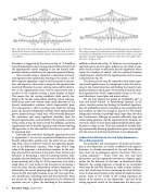
Fig. 4. Illustration of the method for determining a localized eigenfunction from the value and first derivative of the eigenfunction at a point (at the center in the illus- trations). (a) Using exact values and math theorems. (b) Using a numerical method in a computer.
directions, as suggested by the arrows in Fig. 4a. It should be noted that having the exact starting value and first derivative of the eigenfunction causes coupling to just the linearly inde- pendent solutions which have the required exponential decay.
Now consider using a computer to determine the local- ized eigenfunction numerically. Starting at the center, a reli- able computer algorithm10 may be used to proceed in the pos- itive and negative x-directions to compute the eigenfunction iteratively. However, the exact starting value and first deriva- tive of the eigenfunction must now be represented with a number in the computer having a finite number of digits. This means that the starting condition, while mostly cou- pling to the linearly independent solutions which exponen- tially decay, must now contain some small admixture of the linearly independent solutions which exponentially grow. The consequence is that in moving away from the starting point, the linearly independent solution which exponentially grows, despite having a small start, will eventually dominate the calculation and cause significant deviation from the desired eigenfunction, as illustrated by the upward curvature of the arrows in Fig. 4b. How to avoid this problem, and more significantly, how to find the eigenfunction without knowing the eigenvalue or the value and first derivative at a point, will be presented next.
Ironically, the method for finding the eigenfunction (and its eigenvalue) is to turn the exponential dominance of one linearly independent solution over the other into an advan- tage. First, select an arbitrary value for the eigenvalue param- eter in the differential equation. Next, begin with a large value of the argument x and arbitrary numbers for the start- ing value and first derivative at this point. Then iterate in the direction of decreasing x until the growing linearly inde- pendent solution dominates. This process is illustrated by the arrows pointing left in Fig. 5a. At the same time, start with a small value of x and iterate in the direction of increasing x until the other linearly independent solution dominates, as indicated by the arrows pointing right in Fig. 5a. At the point where the left and right iterations cross, the true eigenfunc- tion should have a matching value and first derivative. Since our choice for the eigenvalue parameter in the differential equation was just a guess, the matching of the iterations is
unlikely, as illustrated in Fig. 5a. However, we can change the eigenvalue guess and try again. Indeed, we can utilize a com- puter search routine to efficiently find the eigenvalue which causes the iterations to match, with the matched iterations comprising our solution for the eigenfunction; such a success is illustrated in Fig. 5b.
The above process may be repeated to find other eigen- values and eigenfunctions. It is important to note that by iter- ating in the inward direction and finding the linearly inde- pendent solutions which grow, we fortuitously find the local- ized eigenfunction which exponentially decays in the out- ward directions, toward plus and minus infinity.
We can now address the notion of “probability one” at “plus and minus infinity” in Furstenberg’s theorem. In the reverse iterative process for finding the localized eigenfunc- tion, the probabilistic nature is manifest in the assumption that the iterations are taken far enough so that one of the linearly independent solutions is probably much larger than the other one. Furthermore, although we needed sufficiently large and small starting positions x for the arguments in the iteration, the system for which we have found exponentially localized eigen- functions is finite in size. Thus this method for actually find- ing exponentially decaying eigenfunctions gives some insight into the nature of Anderson localization in one dimension.
Anderson localization in two and three dimensions— The scaling argument
The properties and consequences of Anderson localiza- tion in one dimension are firmly established with rigorous theorems. As already mentioned, in two and three dimen- sions there are no analogous rigorous theorems. There is a “scaling argument”11,12 which treats one, two, and three dimensions, and this argument provides an adequate expla- nation for the behavior of electrons in disordered solids. However, the scaling argument is based on an assumption which may be valid for electrons in solids at finite tempera- tures, but which may be less convincing for ideal (lossless) waves in disordered systems in the regime of Anderson local- ization. Some of the results of the scaling argument are known to be incorrect in one dimension,13 and one of the scaling argument results in two dimensions has been ques-
16 Acoustics Today, January 2010
Fig. 5. Illustration of the numerical method for finding eigenvalues and eigenfunc- tions using a computer. The method iterates inward and finds solutions which grow into dominance, although the iterations may not match in the middle, as in (a). The eigenvalue is found by requiring the iterations to match their value and first deriv- ative upon crossing, as in (b).