Page 12 - Acoustics Today

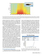
Fig. 4. Composite spectrogram showing the night time fish chorus in Charlotte Harbor, Florida. Each vertical band represents acoustic energy recorded in a 10 second file, with files recorded every 10 minutes. Early in the evening around 1900 hrs sound production begins with sand seatrout producing a purring sound. They are joined later with the higher frequency chatter sounds produced by silver perch. Ambient sound levels increase about 40 dB nightly due to fish sounds over a period of about 6 months. Photo of silver perch: National Oceanic and Atmospheric Administration (NOAA).
spawning in these species. Luczkovich et al. (1999) showed that they could locate areas and times of spawning of weak- fish by combining mobile passive acoustic recordings with plankton tows to catch eggs. Aalbers (2008) showed that field-penned white seabass produced the greatest amounts of sound at the times of spawning (See Fig. 4).
The mobile hydrophone mapping technique has been used to map sound-producing fish distributions across entire estuaries, such as Tampa Bay, the largest estuary in Florida (Walters et al., 2009). More recently, effort has gone into the development and use of autonomous passive acoustic recorders. These recorders use flash memory to record sounds, usually at intervals. Since most fish sound produc- tion is frequent, recordings at intervals are sufficient to char- acterize daily and seasonal patterns in sound production (Locascio and Mann, 2008). The main advantage of autonomous recorders is that they enable recordings to be made over large spatial and temporal scales. Now you can be at more than one place at one time, in any kind of weather. Even in hurricanes, which don’t put a damper on fish sound production (Locascio and Mann, 2005) (See Fig. 5).
Can we use sound levels to estimate the number of fish calling in an area? So far, not yet. To do this requires knowl- edge of source levels, calls rates, and propagation loss. This will require collaboration between biologists and acoustic model- ers. The source levels of only a handful of species of fishes have been measured in the field. Some species, like the black drum have source levels up to 160 dB re: 1μPa (Locascio and Mann, 2011). Other fishes have source levels ranging from 125–135 dB re: 1μPa (oyster toadfish: Barimo and Fine, 1998, silver perch: Sprague and Luczkovich, 2004). Many fishes chorus, with so many individuals calling at once that it is not possible to separate sounds from different individuals.
Passive acoustics in ocean observatories
Long-term recorders are yielding insight into the timing of sound production and how it is affected by environmental
factors. A good example of this is acoustic recordings from the LEO-15 ocean observatory off the coast of New Jersey. The continental shelf off New Jersey experiences high annu- al temperature variations and is highly dynamic. Sound pro- duction by chorusing croakers and weakfish varied in close concert with upwelling events, where sound production ceased as cold water invaded the observatory (Mann and Grothues, 2009). While it is not known whether the fish ceased producing sound or moved to another location, pas- sive acoustics provided a means to study behavior on the same time scale as oceanographic events (See Fig. 6).
New buoyancy propelled electric gliders allow longer missions under a lower power budget than autonomous underwater vehicles (AUVs), and are potentially much qui- eter, since there is no mechanical propeller. Gliders are an important part of the development of ocean observatories
Fig. 5. History of capabilities of acoustic recorders used over the past 17 years. Recorders have evolved from intelligent real-time detection of specific sounds to high sample rate, large memory capacity recorders. The new challenge is now analyzing large acoustic datasets.
Remote Sensing of Fish 11