Page 28 - Acoustics Today

major differences in the marine environment between the locations where the forward and inverse problems are used (Warren and Wiebe, 2008).
Many of these complications and difficulties are beyond our control as scientists. The ocean is a dynamic environ- ment; nekton and zooplankton occur in patches so their abundances can vary over several orders of magnitude over very short time and space scales (minutes, 10s of meters); using ship-based platforms makes it difficult to make synop- tic measurements (unlike satellites); and there are many fac- tors which can affect the target strength of a particular species (size, orientation, health/fitness). So uncertainties in acoustic estimates can be quite large. However despite these issues, inversion of acoustic data for biological information is done accurately over both large and small scales throughout the world. Many fisheries throughout the world use acoustic methods accompanied by net and trawl sampling to produce a stock assessment for management purposes including sev- eral of the largest in terms of landings such as pollock, hake, herring, sardine, and anchovy. Historically, there have been technological reasons (as opposed to our general ignorance about how the natural world works) that limited our ability to accurately measure these systems; however that is changing.
Mo’ beams; mo’ bandwidth; mo’ data
Traditional fishery echosounders operate at a single acoustic frequency between 10 and 200 kHz with narrow bandwidth (< 10%) and beamwidths between 7 deg and 30 deg, and are hull-mounted pointing downward. Thus as ship moves around, data are collected in a cone beneath the ship producing a ribbon-like plot of acoustic backscatter (Fig. 1). Many fishery survey vessels travel ~ 10 kts so covering a large habitat area will take several weeks or months at sea and pro- duces transect lines that are widely spaced often several km apart. While a great improvement in terms of spatial and tem- poral coverage relative to other sampling systems, these sur-
veys still cover a relatively small volume of the marine habitat. When a fish school is measured by a traditional echosounder, we know the vertical dimension (height) of the school along the ship’s path; however we do not have any information as to the cross-track dimension of the school. One can make assumptions as to whether fish schools are isotropic or not, but our picture of the size of a fish school is incomplete.
Multibeam acoustic systems, originally developed for high-resolution bathymetric mapping, have changed our data collection from being a 2-D system (depth, distance along the ship’s path) to a 3-D system (depth, along- and cross-path dis- tance) greatly increasing the volume covered in an acoustic survey (McGehee and Jaffe, 1996; Jaffe, 1999). Unlike tradi- tional echosounders, multibeam systems provide cross-track information as to fish school dimensions and in some cases entire fish or zooplankton schools can be ensonified. (Weber et al., 2009; Cox et al., 2009; Cox et al., 2010). Studies have even been able to show feeding interactions between groups of air- breathing predators whose lungs scatter significant amounts of energy and schools of their prey (Benoit-Bird and Au, 2009; Benoit-Bird, 2009b). Many countries that regularly conduct fishery surveys are equipping their fleets with these systems, along with the traditional echosounders, to take advantage of the increase in sampling volume. However, there are some new problems that have arisen with these systems. Calibration of a multibeam system can be challenging (Foote et al., 2005) and some animals will scatter sound differently depending on their orientation relative to the acoustic transducer. Two identical scatterers (size, species, orientation) may have different target strengths depending on whether they are ensonified by a beam directly above them or from a beam off to their side (Roberts and Jaffe, 2008).
Shifting from using a single frequency to multiple fre- quencies of sound to survey the ocean is analogous to view- ing a picture in black and white and then adding additional colors to the image (Gareth Lawson was the first person I
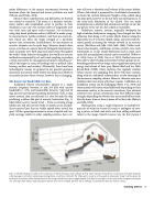
Fig. 1. A 200 kHz echogram recorded in the coastal waters of Alaska showing a school of Pacific herring. Colors represent strong (brown and red) and weak (blue and green) scattering regions with white representing scattering below an arbitrary threshold. The ribbon-plot is made up of thousands of echosounder “pings” which measure the backscatter in the water column beneath the boat. The strong red and brown layer at approximately 50 m depth is the seafloor. As our vessel moved we appear to have gone over a herring school (likely a single school given that the area shown is roughly 100 m by 150 m, although it is possible that they were distinct schools).
Counting Critters 27