Page 29 - 2016Fall

into account when designing systems and experiments. I have seen it many times.
Horror Story About Observability
I was invited to work on a multiyear project that was nearing completion. The goal was to use a cubic array of six acceler- ometers to replace gyroscopes in a space vehicle. Six accel- erometers were used because the system kinematics could be modeled as a sixth-order nonlinear ordinary differential equation (ODE). Later, the team realized that ODE solvers do not work well with noisy measurements, so I was asked to build a recursive estimator for the linear and angular veloci- ties of the vehicle. A two-axis magnetometer was available but could only measure two angular velocities. I showed that the system was not observable because not enough measure- ments were available to estimate the six system states. All I could do was build an extended Kalman filter and use simu- lations to show what could have been done if enough mea- surements had been available.
Gaussianity
Measured signals are modeled as stochastic processes with particular probability density functions (Papoulis and Pillai, 2002). Many (if not most) signal processing algorithms are derived assuming that the stochastic processes are Gaussian distributed, mostly because the Gaussian assumption makes algorithm derivation mathematically tractable. In real-world applications, however, we often measure non-Gaussian dis- tributed signals that must be processed.
In my experience, very few people ever test their signals for Gaussianity. Most people go ahead and apply algorithms de- rived for Gaussian signals without giving the data distribu- tion any consideration. Later, they wonder why the signal- processing algorithms produced poor results. I advocate that the data should be tested for Gaussianity at the beginning of the project (Crawley, 2012; Clark, 2014).
Stationarity
Many signal-processing algorithms are derived assuming that the signals are statistically wide-sense stationary (Pa- poulis and Pillai, 2002). Many problems are caused when people apply these algorithms to nonstationary signals. A real stochastic process x(t) is called wide-sense stationary if its mean (expected value) is constant, E{x(t)}= η, and its au- tocorrelation R(τ)=E{x(t)x(t+τ)} depends only on the time shift τ = t1–t2 . Clearly, transient signals (e.g., broadband pulses) are not stationary, yet we routinely process transient
signals using algorithms derived for stationary signals be- cause these algorithms are tractable. However, we must un- derstand that the processing results may be surprising and/ or not useful (Candy et al., 1986).
Inverse Problems
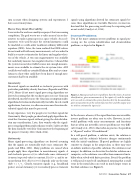
Two of the most common inverse problems in signal pro- cessing are the system identification and deconvolution problems, as depicted in Figure 2.
Figure 2. Many practical inverse problems have this form. In system identification, given measurements of the input x(t) and the output u(t), we wish to estimate the system function h(t). In deconvolution, given measurements of the system function h(t) and the output u(t), we wish to estimate the input x(t) .
In the absence of noise, if the signal functions are invertible, inverse problems are often easy to solve. However, in real- world problems with noisy measurements and functions that are often not invertible, inverse problems are very diffi- cult (Candy et al., 1986). Most often in practice, the problem is “ill posed” and/or “ill conditioned.”
In a well-posed problem, a solution exists, the solution is unique, and the solution’s behavior changes continuously with the initial conditions. Ill-posed problems are highly sensitive to changes in the output data, so there may exist an infinite number of possible solutions (the solution is not unique). In addition, we discretize the data for solution on a computer, so the solutions can suffer from numerical insta- bility when solved with finite precision. Even if the problem is well posed, it may be ill conditioned, meaning that a small error in the initial data can result in much larger errors in the final solutions (see Figure 3).
Fall 2016 | Acoustics Today | 27