Page 24 - 2016Winter

Maxwell and Acoustics
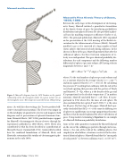
Figure 2. Maxwell’s diagram from his 1873 Treatise on the spatial relationship of the electromagnetic fields “at a given instant” for an electromagnetic wave. This image was scanned from an 1892 printing.
nions. (As with his other writings, his Treatise predated effi- cient vector and tensor notation.) The Treatise was unique in its liberal display of quantitative electric and magnetic field diagrams and its presentation of spherical harmonic func- tions. Heinrich Hertz (1857-1894) provided major support for Maxwell’s electromagnetic theory of waves through his experiments published in 1888 (Hertz, 1893). Hertz also contributed to what has been described as a purification of Maxwell’s theory (Sommerfeld, 1952). Sommerfeld recalled how the combined formulations of Maxwell, Hertz, and Heaviside systematized the totality of electromagnetic phe- nomena in the early 1890s.
elastic spheres that interacted only during collisions. In the absence of flow of the gas, Maxwell postulated that after the collision of spheres, the three Cartesian components of ve- locity were independent. This gave identical probability dis- tributions for each component and the following number differential of spheres (per unit volume; dN) having velocity magnitudes between v and v + dv
dN = 4N α−3π−1/2v2 exp(−v2/α2) dv (1)
where N is the total number of spheres per unit volume and α is a constant related to the average velocity (<v> = 2απ−1/2) and mean squared velocity [<v2> = (3/2) α2]. By calculating the pressure (P) resulting from collisions with the side of the vessel and equating that pressure with the gas law of “Boyle and Mariotte,” P = Kρ, where ρ is the density of the gas and K is proportional to the absolute temperature (T in modern notation), Maxwell concluded that α2 = 2K. Here, K is pro- portional to T/M, where M is the mass of each sphere. He also concluded that for a given P and T, NM<v2> is the same for all gases. By that stage of his paper, Maxwell had sepa- rately concluded that (M/2)<v2> is the same for differing sets of spheres in equilibrium (an energy equipartition theorem) and hence that his model explained the observed behavior of gases. Using modern terminology, Equation 1 is an example of a Maxwell-Boltzmann probability distribution.
Some of the other quantities examined by Maxwell depend on the size of the colliding gas particles through (in his no- tation) s, the sum of the radii of the colliding spheres. For simplicity in what follows, attention is restricted to the situa- tion of identical spheres. Maxwell found that the “mean path of each particle” (L) between collisions was L = 1/(Ns2 π21/2).
Maxwell’s First Kinetic Theory of Gases, 1859, 1860
Between the early stages of his development of electromag- netic theory, Maxwell initiated a quantitative formulation of the kinetic theory of gases by introducing probabilistic distributions into physical theory. He also provided a physi- cal basis for modeling transport coefficients (Garber et al., 1986). The principal publication (Maxwell, 1860) expanded on his presentation at the 1859 meeting of the British As- sociation for the Advancement of Science (BAAS). Maxwell
modeled a gas as if it consisted of a large number of hard
Replacement Equation page 22
22 | Acoustics Today | Winter 2016