Page 35 - 2017Winter

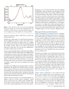
Figure 5. Power spectrum of the cosmic microwave background fluctuations. Angular size is the most interesting quantity here. The multipole moment (l), which is a more proper mathematical descrip- tion, is simply given by 1~180 (angular size). Courtesy of NASA.
sponds acoustically to about 110 dB. These are fairly sub- stantial sound waves!
Perhaps more importantly, the small density disturbances shown in Figure 4 are pictures of the seeds of future struc- ture. Galaxies and clusters of galaxies that are a million times denser than the universe’s mean density formed from the overdense regions, whereas vast cosmic voids formed from the less dense parts. The exact way this “amplification” occurred is still an active research area.
To get at some of the other physics contained in the CMB, we need to further distill the spatial image seen in Figure 4 into a spatial power spectrum. This means doing a decomposi- tion similar to the spherical harmonic analysis that was done for helioseismometry. (Only because space is basically iso- tropic, we don’t have the north-south versus east-west dis- tinction we have for the sun. So there is one less modal index to consider.) A power spectrum versus angular size is shown in Figure 5.
The peaks in the CMB power spectrum contain a wealth of information. The angular scale of the first peak is a measure of the curvature of the universe and says (in good agreement with inflation theory) that the universe has a flat geometry. The ratio of the next peak to the first (or odd-to-even peaks in general) gives the baryon density, whereas the third peak informs about the dark matter density.
Another acoustic result that is very useful in modern cos- mology is how the “baryon acoustic oscillations” (sound waves) we discussed create a rather useful “standard ruler” for the universe. If one considers a single acoustic wave from an overdense region originating in the center of the primor-
dial plasma, it is easy to show that at the time of decoupling/ recombination, when the photons start moving away from the baryonic matter, there is an overdense shell of this mat- ter left at a fixed radius. This radius is called “the sound hori- zon,” and as a result of it, when the universe evolves further, cosmologists expect a local maximum in the number of gal- axies separated by that scale. That is indeed what was found by the Sloan Digital Sky Survey of galaxies and confirms the CMB observations that the sound horizon is ~150 megapar- secs (1 parsec = 3.2 light years), which can then be used as a standard ruler. This ruler, combined with the CMB observa- tions, can be used to study the mysterious “dark energy” that seemingly comprises 70% of our universe (Morgan, 2014)!
Seeing with Sound: Sonification
Another astronomical use of sound is its use in “visualizing” various types of data that have features that are sometimes better detected by our ears than by our eyes. As an example, our eyes can detect differences in images that are presented at a frame rate of about 50 Hz, but our ears can sense up to 20 kHz. Also, our ears can be sensitive to nuances that are not readily visible in time series plots or spectra; the brain has some very good signal processing capabilities! Sound is also something we can viscerally relate to, especially if we turn up the bass! So data on many of today’s astronomical phenomena have been “translated” into sonic representa- tions. Let’s look at a few.
Perhaps the most famous recent sonification has been from the Laser Interferometer Gravitational Wave Observatory (LIGO) observations of merging black holes. These as- tounding observations actually show gravity wave arrivals that occur in the same frequency range as acoustics and so are natural candidates for sonification. The first obser- vations showed a 0.2-second up-chirp that one could hear easily at the original frequency and when slightly shifted up in frequency sounded like a bird chirp. The two sub- sequent observations also show a similar structure (as the black holes spiral in faster and faster). (For example, see http://acousticstoday.org/bh).
Another favorite sonification is “the sound of the big bang.” A nice example of this can be found on the web- site of John G. Cramer of the University of Washington (http://acousticstoday.org/cramer). It is based on models of the universe’s evolution over a 760,000-year time period that are constrained to correctly describe the CMB spectrum that is seen in Figure 5. As the universe expands, it becomes more and more of a bass instrument (which reflects the
Winter 2017 | Acoustics Today | 33