Page 74 - Spring2019

Student Challenge Problem
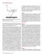
Figure 1.Contributions to the underwater sound field from an airborne source. After Urick (1972).
of the aircraft. The base of the cone subtends an apex angle, which is twice the critical angle, and the height of the cone corresponds to the altitude of the aircraft.
The first activity of the Student Challenge Problem is to test the validity of Urick’s model for the propagation of a tone (constant-frequency signal emitted by the rotating propeller of the aircraft) from one isospeed sound propagation medi- um (air) to another isospeed sound propagation (seawater), where it is received by a hydrophone. Rather than measuring the variation with time of the received acoustic intensity as the acoustic footprint sweeps past the sensor (as Urick did), it is the observed variation with time of the instantaneous frequency of the propeller blade rate of the aircraft that is used to test the model. This is a more rigorous test of the model. The frequency of the tone (68 Hz) corresponds to the propeller blade rate (or blade-passing frequency), which is equal to the product of the number of blades on the propeller (4) and the propeller shaft rotation rate (17 Hz). For a turbo- prop aircraft, the propeller blade rate (or source frequency) is constant, but for a stationary observer, the received fre- quency is higher (commonly referred to as the “up Doppler”) when the aircraft is inbound and lower (“down Doppler”) when it is outbound. It is only when the aircraft is directly over the receiver that the source (or rest) frequency is ob- served (allowing for the propagation delay). The Doppler ef- fect for the transit of a turboprop aircraft over a hydrophone can be observed in the variation with time (in time steps of 0.024 s) of the instantaneous frequency measurements
of the received signal, which is recorded in the file Time vs. Frequency Observations. This file can be can be down- loaded at acousticstoday.org/iscpasp2019. The first record at time −1.296 s and frequency 73.81 Hz indicates that the air- craft is inbound, and for the last record at time 1.176 s and frequency 63.19 Hz, it is outbound.
Task 1
Given that a turboprop aircraft is in level flight at a speed of 239 knots (123 m/s) and an altitude of 496 feet (151 m); that the depth of the hydrophone is 20 m below the (flat) sea sur- face; that the isospeed of sound propagation in air is 340 m/s; and that in seawater, it is 1,520 m/s, the students are invited to predict the variation with time of the instantaneous fre- quency using Urick’s two isospeed sound propagation media approach and comment on its goodness of fit to the measure- ments in the file.
Task 2
Figure 2 is a surface plot showing the beamformed output of a line array of hydrophones as a function of frequency (0 to 100 Hz) and apparent bearing (0 to 180°). This plot shows the characteristic track of an aircraft flying directly over the array in a direction coinciding with the longitudinal axis of the array. The aircraft approaches from the forward end-fire direction (bearing 0°; maximum positive Doppler shift in the blade rate), flies overhead (bearing 90°; zero Doppler shift), and then recedes in the aft end-fire direction (180°; maxi- mum negative Doppler shift). For this case, the bearing cor- responds to the elevation angle (ξ), which is shown in Figure 3, along with the depression angle (γ) of the incident ray in air. The (frequency, bearing) coordinates of 32 points along the aircraft track shown in Figure 2 are recorded in the file Frequency vs. Bearing Observations, which can be down- loaded at the above URL. Each coordinate pair defines an acoustic ray. Similar to the previous activity, for Task 2, the students are invited to predict the variation with the eleva- tion angle of the instantaneous frequency of the source signal using Urick’s two isospeed media approach and to comment on its goodness of fit to the actual data measurements. The aircraft speed is 125 m/s, the source frequency is 68.3 Hz, and the sound speed in sea water is 1,520 m/s.
Task 3
To replicate Urick’s field experiment, a hydrophone is placed at a depth of 90 m in the ocean and its output is sampled
72 | Acoustics Today | Spring 2019