Page 24 - Spring2020

Synthesis of Musical Instrument Sounds
synthesized by a deep neural network. This minimization process is carried out by means of some (typically gradient- based) optimization procedure applied to some metric or loss function. Thus, the development of NAS models obviates the need for explicit physics-based models, instead requiring a
“training dataset” of prerecorded audio sounds against which to refine the model’s outputs. Rather than relying on physi- cally relevant control parameters, NAS models may “learn” alternative parameterizations of the sound.
NAS architectures have primarily taken the form of autoen- coders or Generative Adversarial Networks (GANs), which we describe shortly. An attractive feature of these two archi- tectures is that they are “unsupervised” (or “self-supervised”) learning models for which the algorithm does not require human labeling of their datasets, an enterprise that can suffer from expenditures of time and finances or concerns about accuracy.
Autoencoder Approaches
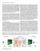
An autoencoder is a deep neural network trained to reproduce its input. It consists of multiple layers of artificial neurons arranged in an encoder-decoder pair (illustrated in Figure 3). The “hourglass” shape of the autoencoder forces the model to “learn” a compressed parameterization, often referred to as a “latent space representation” (i.e., Figure 3, center of hour- glass), for determining the output signal. This reduced set of encoded features can then be altered slightly and decoded to synthesize new forms of audio, that is, one can later use the decoder portion alone as a synthesizer. The encoder and
decoder may consist of one or multiple layers of neural con- nections, which can allow differing hierarchies of modeling complexity (see Roche et al., 2018, for a comparison). The inputs and outputs of the autoencoder may be raw audio waveforms, so-called “end-to-end” models, but more typically are magnitude spectrograms obtained via short-time Fourier transforms (STFTs) or related transformations. To produce the final waveform from the output spectrogram, there are well-known iterative techniques that can be used (Griffin and Lim, 1984). The hidden layers within the encoder and decoder may be simple “fully connected” layers (i.e., matrix multiplications followed by nonlinear activation potentials) or may involve structures that allow for more efficient cap- turing of behavior over “long” timescales, such as recurrent neural network layers with an internal memory (Mehri et al., 2016), or a stacked series of dilated convolutions as in the WaveNet scheme (van den Oord et al., 2016).
A noteworthy end-to-end autoencoder model known as NSynth was created in the Google Magenta group (avail- able at tinyurl.com/gmagenta; Engel et al., 2017). This group trained two different autoencoder models on an extremely large dataset of musical instrument sounds consisting of
“~300k four-second annotated notes sampled at 16 kHz from ~1k harmonic musical instruments.” They compared the performance of a baseline spectral autoencoder model of the type described above with an autoencoder that used a WaveNet structure, finding the latter offering significant improvements in reproducing aspects of tone quality, attack transients, timbre, and dynamics. The latent-space encod-
Figure 3. Schematic of an autoencoder method in which the output spectrogram of a neural network approximates its input spectrogram. Here we show fully connected neural network layers operating on spectrograms, whereas other autoencoders make use of more complex network architectures (e.g., recurrent or convolutional neural network layers) and operate directly on raw audio.
24 | Acoustics Today | Spring 2020