Page 63 - Summer 2021

These two equations correspond to Eqs. 6 and 7, respec- tively, in Stanton et al. (2018) but with a change in notation. The term fb(si) is the backscattering amplitude of the ith scatterer, b(θi, φi) is the beampattern function of the sensor system as evaluated at the location of the ith scat- terer in the beam, (θi, φi) are the spherical polar angular coordinates of the scatterer in the beam, Δi is the total phase shift associated with the ith scatterer (phase associated with scattering properties, the distance between the sensor and scatterer, and the beamformer) and j = √−1. The term fb(si) represents the efficiency with which the object scatters a signal and its magnitude is equal to the square root of the differential backscattering cross section. The phase shift term Δi is the source of interference between different scat- terers, which contributes significantly to echo fluctuations.
Equations 1 and 2 are for acoustic and electromagnetic waves that have a long duration and are at a constant single frequency, scatterers that are within a narrow range of distances from the sensor system, assume a direct path between the sensor system and scatterer (no boundaries or variations in environmental properties), and are for first-order scattering only. Constants of the system, such as system gain, have been suppressed for convenience. These simple equations describe scalar waves where shear waves (acoustic) and polarization effects (electromagnetic) are not accounted for. Details of these equations are in Stanton et al. (2018), where more complex and realistic scenarios are also described.
Each of the following three terms in Eqs. 1 and 2 are considered in this analysis to be random variables: fb(si) varies with random orientation and size, shape, and mate- rial properties of the scatterers; b varies with the scatterers’ random angular location (θi, φi) in the beam; and Δi varies with scatterer properties and random range. For simplicity, the number of scatterers (N) in each transmission is held fixed, although that term can also be randomized to simu- late a non-uniform distribution of scatterers. Because the above three terms are random variables, the echo ã is also a random variable.
In addition, as the sensor system scans an area, different scatterers are “seen” by the system from transmission to transmission. Because naturally occurring objects are generally randomly distributed, the echo will correspond- ingly vary randomly from transmission to transmission according to the complex combination of the scattering,
the random location in the beam, and the interference processes that vary across transmissions. This random variability can be accounted for in Eqs. 1 and 2 through randomizing the three parameters: fb(si), b(θi, φi), and Δi . An ensemble of statistically independent realizations of ã is calculated through the summation in Eq. 1 for a statisti- cally independent set of values of each of the three terms. The probability density function (PDF) of the echoes is formed from the ensemble of the echoes and represents the probability of occurrence of each echo value. This PDF is considered a “physics-based” model because the scatterer properties and sensor properties are explicit in the formula- tion. Its shape and mean value vary with those properties.
Connecting Theory with Experiment
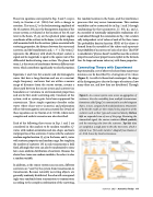
Experimentally, a set of observed echoes from many trans- missions can be described by a histogram of its values (Figure 2). As with its theoretical counterpart, the shape of the histogram gives clues to the types of scatterers, how many there are, and how they are distributed. Through
Figure 2. As a sensor system scans across an aggregation of scatterers, the echo variability from multiple transmissions (sometimes called “pings”) is summarized in an echo histogram that is, in turn, compared with model predictions. Parameters of the best fit model are then related to key properties of the scatterers such as their type and numerical density. Bottom left: an expanded view of one of the pings illustrating the transmitted signal, the various scatterers (black symbols), and the returning echo from the scatterers. Top left: data are sampled at a single point in the echo time series, which is referred to as “first-order statistics.” Adapted from Stanton et al., 2018, license by Creative Commons.
Summer 2021 • Acoustics Today 63