Page 26 - Spring 2007

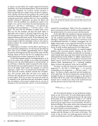
Fig. 18. Finite element predictions for the first two mode shapes and resonance fre- quencies of a thin shell. The rigid ends on both sides of the shell simulate semi-infi- nite rigid baffles.
an infinite circular baffle. For simply-supported boundary
conditions, the structural displacements can be determined
analytically. Similarly, the acoustic Green’s function is
known analytically for a simple source outside of a rigid cir-
cular cylinder, and thus for this problem the acoustic field
can also be determined analytically, although it can only be
evaluated numerically. Solutions for the in vacuo and fluid-
coupled resonance frequencies are given by Berot and
23
Peseux.
For this problem, the cylinder has radius 0.4 m,
length 1.2 m, and is 3 mm thick. Its material properties are
given as E = 200 GPa, ρ = 7850 kg/m3, v =0.3, and the sur-
rounding water has properties cο = 1500 m/s, and ρο = 1000
3
kg/m . We note that the thickness–to-radius ratio is less
than 0.01 for this example, and thus thin shell theory is applicable and we expect a relatively large shift in the reso- nance frequencies due to fluid-loading. Our goal will be to reproduce Berot and Peseux’s results. In the numerical com- putations, the structural analysis proceeds as usual, but we cannot simply model the boundary surface in the acoustic analysis because the circular baffle extends to infinity in both directions.
Following the procedure used by Berot and Peseux in their numerical computations, we will truncate the baffle on both sides of the cylinder approximately half its length beyond the vibrating portion and close off the ends with flat endcaps. Figure 18 shows the first two computed in vacuo mode shapes and resonance frequencies for the shell.
In the finite element analysis, the displacement is set to zero at the ends of the cylinder in the radial and torsional directions, but the axial displacement is unconstrained. As we will show, a fairly fine mesh is required in the circum- ferential direction to properly represent the acoustic imped- ance of the higher order modes. For example, to correctly represent a mode with 8 circumferential wavelengths, we need (8)(6)=48 acoustic elements around the circumfer- ence. The acoustic mesh does not have to be nearly as refined in the axial direction because the structural stiffness is much higher. With this in mind, the structural mesh has 24 elements in the axial direction and 48 elements around the circumference. The acoustic meshes have 8, 12, and 12 elements in the axial direction, and 16, 24, and 48 elements
around the circumference. Table 2 lists the resonance fre- quency ratios given by Berot and Peseux along with numer- ical predictions for the various acoustic element meshes.
In the table, NA is the number of acoustic elements for each of the boundary element meshes. Clearly, the numeri- cal and analytical predictions match each other closely, although a relatively fine acoustic mesh is necessary in the circumferential direction to achieve convergence for the higher order modes, as was expected. Overall, for structures submerged in water, the fluid-loading analyses has been shown to yield excellent predictions for the added mass.
We consider a cavity-backed plate as a second example problem with structural-acoustic coupling. In the 1970’s, Guy and Bhattacharya24 studied transmission loss through a cavity-backed finite plate and their results have been used subsequently by several authors to validate numerical pre- dictions. We will similarly use the problem to illustrate how dipole sources can be used to model interior and exterior acoustic fields simultaneously in a scattering problem. Figure 19 shows the geometry of the cavity and plate.
The plate is 0.914 mm thick and is made of brass with
properties E = 106 GPa, ρ = 8500 kg/m3, v = 0.3, and the
. (31)
For the numerical analysis, we can perform the compu- tations in one of two ways. We could simply apply mechan- ical forces to produce a uniform pressure to the top surface
25
face mesh with 864 structural elements.
The incident pressure is computed knowing the source
location and the distance to the center of the plate. The results in Fig. 20 show very good agreement between our numerical predictions and Guy and Bhattacharya’s experi-
surrounding air has properties cο = 340 m/s, and ρο = 1.2 3
kg/m . The plate is simply-supported and the backing cavi- ty has rigid walls. We want to compute the transmission loss through the plate to a field point location at the center of the back wall of the cavity. Guy and Bhattacharya’s trans- mission loss is actually just a ratio of the incident pressure and the pressure near the back wall of the box:
and M. Guerich and M. A. Hamdi,26 or we could simulate the exper- iment using an acoustic source as the excitation. We will use the latter method. The surface of the cube is divided evenly into 144 quadrilateral elements, yielding a boundary sur-
of the plate, as in the studies by S. Suzuki, et al.
Table 2. Analytical and numerical predictions for the resonance frequency ratios (in fluid/in vacuo) of the circular shell. Mode orders are indicated as (m,n) pairs, where m is the order along the axis, and n is the circumferential harmonic.
24 Acoustics Today, April 2007