Page 25 - Spring 2007

benefited enormously from the rapid increase in computer processor speed and memory. Since boundary element com- putations are repeated many times at different frequencies, it is easy to split jobs up and assign them to different comput- ers or processors.
In practice, boundary element methods are very compet- itive for all but the very largest engineering problems, where the matrix inversion and multiplication dominate the solu- tion times. This is especially true if the time required to cre- ate models is factored into the analysis. In this respect, boundary element methods are relatively quick and easy. Simple rules of thumb can be used to determine if boundary element methods will be applicable for a specific problem. Generally, six elements are required per acoustic wavelength to accurately compute an acoustic field. Knowing the surface area S of the boundary and the maximum frequency of inter- est, the required number of acoustic elements is given as S/(π/3fmax)2. Three matrices of this size will be required to compute the matrix multiplication, and it is usually best to do the computations in double-precision, thus requiring 16 bytes for each element of the matrices.
Modeling sound—structure coupling
Recall that a moving structure compresses and contracts neighboring fluids, which act as a continuous elastic blob around the structure. When the fluid is heavy, its pressure loading affects the structural vibrations. To compute these effects, the boundary element model must be coupled to a representation of the structure.
The previous analysis has shown that an acoustic imped- ance matrix, relating the pressures to the normal component of velocity on the boundary surface, can be computed as a function of frequency using boundary element methods. We now want to combine this result with a finite element analy- sis of the structural vibrations to include the effects of the pressure field. In a finite element analysis, the displacements are written in the form
, (29)
where M, B, and K are the mass, damping, and stiffness matrices, d is the displacement field of the structure, and F is the vector of forces applied to the structure.
To include the pressure field in the finite element analy- sis, the impedance matrix must be transformed from its dependence on normal surface velocity to nodal displace- ments. For time-harmonic problems, the displacement field on the outer surface of the structure can be used to compute the normal component of the surface velocity as a simple dot- product: vn = v . n = -iω d . n. Thus, a matrix relationship can be derived to convert the complete displacement field into a normal surface velocity vector. This matrix will have zeros for all interior nodes not in contact with the surrounding fluid. Similarly, the matrix will also be zero for displacement degrees of freedom on the boundary surface tangential to the outward surface normal. Post-multiplying the acoustic impedance matrix by the transformation matrix then yields a matrix relationship between the pressure field on the bound- ary and the finite element displacement vector. Including the
result for the pressure field on the boundary surface in the finite element equations of motion yields
. (30)
Given an input force vector, it is theoretically possible to solve this equation for the displacement vector, which now includes fluid coupling. In a finite element analysis, the equa- tion system is highly-banded because each element only interacts with other elements through the nodes. However, in a boundary element analysis, every node interacts with every other node, so that the acoustic impedance matrix is general- ly fully-populated. It then becomes very time-consuming to solve the matrix system in its present form. Various alterna- tive strategies are possible where the matrices are subdivided into degrees of freedom with and without fluid coupling. It is also possible to treat the acoustic pressure field on the
21
Ultimately, many researchers instead reformulate the problem in terms of a modal frequency response analysis (which is the approach we use at Penn State). In a modal frequency response, the mass, damping, and stiffness matrices are pre- and post-multiplied by mode shapes, and the applied force vector is pre-multi- plied by the mode shapes. The resulting system, which is usu- ally much smaller in size than the system defined in physical coordinates, is solved to compute modal coefficients. The modal coefficients tell us how much each mode contributes to the overall response, and are multiplied by the mode
boundary surface as the primary variable.
shapes to compute that physical response.
Using the coupled FE/BE formulation, the time required
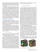
to compute and store the acoustic impedance matrix as a function of frequency typically dominates the overall solu- tion times. To speed up this part of the process, it is common to condense the structural displacement variables into a coarser set of acoustic variables. To illustrate, Fig. 17 shows two structural and acoustic meshes for a loudspeaker.
Since both the structural and acoustic fields require approximately six elements per wavelength, this process assumes that the structural waves vary more rapidly than the acoustic waves. This is true below the coincidence frequency, and is valid up to a relatively high frequency for structures submerged in water.
To demonstrate the typical results of a coupled FE/BE analysis, two example problems will be considered. The first is the familiar example of a thin circular cylindrical shell in
Fig. 17. A structural mesh for a speaker with two different acoustic meshes.
Structural Acoustics Tutorial 2 23