Page 13 - Acoustics Today Summer 2011

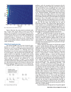
Fig. 2. Measuring the acoustic field in the ocean.
Figure 2 illustrates the ocean acoustics estimation prob- lem. A source emits sound, which is sensed at an array of phones. The array could be a vertical line array (VLA), a hor- izontal line array (HLA), or a more complex configuration of a sensor geometry. We wish to “invert” the measured data for estimation purposes. Parameters to be estimated may include source location, array tilt and shift, sound speed in the ocean and seafloor sediments, sediment thickness, atten- uation, and density.
Model-Based signal processing
The concept of MBP is not a new one, because the spec- ification of a model is required for any inverse problem. However, its use as a means of improving the performance of an ocean acoustic processor is a relatively novel idea. Historically, its use in ocean acoustics probably began with the work of Hinich,5 who showed that by including the prop- agation model in the algorithm, the depth of an acoustic source in an acoustic waveguide could be readily estimated. Bucker6 later showed that both the range and depth of the source could be estimated and introduced the term “Matched-Field processing,” or MFP. A more detailed description of the history and methods of MFP can be found7 in a special dedicated issue of the Institute of Electrical and Electronic Engineers (IEEE) Journal of Oceanic Engineering.
Originally, MFP was applied solely to source localization
Fig. 3. Sequential Bayesian filtering.
problems, under the assumption that the parameters describ- ing the medium are known. Although a great deal was done in the field of MFP for source localization, still a rather useful approach to many ocean acoustic problems, there remains a fundamental problem which plagues it, sometimes referred to as the “Mismatch Problem.” This problem arises from the fact that the solution can be highly sensitive to errors in the model parameters. This is not surprising, because it is the complexity of the model itself that leads to the observability of the desired parameters. Thus, if the model is not correct, it will lead to degradation. Sometimes this degradation can be catastrophic.
Although there have been many approaches to try to rem- edy this, the first major step forward was the work of Richardson and Nolte,8 who, working within a Bayesian frame- work, included a priori probabilities in the MFP algorithm to account for uncertainties in the troublesome parameters. As a result, they obtained posterior probability density functions (PDFs) for source location, which described the uncertainty in the estimation process resulting from the lack of precise knowledge on the propagation medium characteristics.
MFP was soon after extended to inversion for environ- mental parameters. The first such application of MFP was presented by Livingston and Diachok,9 who estimated the under-ice reflection coefficient applying MFP to data and sound propagation models in the Arctic. Inversion for the characteristics of the propagation medium subsequently expanded with estimation of geoacoustic parameters in high-
10-16
in mind—namely Bayesian filtering, Candy and Sullivan17 sought to remedy the mismatch problem by embedding the propagation model into a Kalman filter (KF). This has the advantage of allowing the troublesome parameters to be included as part of the state vector of unknowns, a procedure known as “augmentation.” A further advantage is that the Kalman formalism provides a natural and self-consistent framework for the inclusion of essentially any model. Most subsequent work has improved on this approach, especially by use of the so-called Extended and Unscented Kalman fil- ters18,19 (EKFs and UKFs, respectively) and several variants, and the particle filter (PF),20 the latter pioneered in ocean
ly complex environments.
Within a Bayesian framework, but with dynamic models
21,22
23-26
and subsequently extended. provide a powerful framework for performing signal pro- cessing in nonstationary dynamic systems involving nonlin- ear equations and non-Gaussian PDFs as well as a stream of incoming data. A summary of applications of the family of Kalman and particle filters to problems in ocean acoustics27 is available. These methods are often referred to as sequential Bayesian filtering and rely on a two-stage process. During the first stage, unknown state variables xk at step k are predicted using estimates from step k–1. The second stage entails an update stemming from physical and statistical models that relate acoustic measurements yk to state variables xk. Figure 3 illustrates the two steps of sequential Bayesian filtering. In addition to providing point estimates for the state variables, sequential Bayesian filtering also provides posterior PDFs at
acoustics by Candy
PFs
every step, as will be shown.
Sequential Bayesian filtering has been frequently applied
Model-Based Ocean Signal Processing 9