Page 15 - Acoustics Today Summer 2011

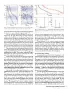
Fig. 7. (a) Synthetic, noise-free time series received at an array of vertically and hor- izontally separated hydrophones; (b) time series after noise has been added.
Fig. 8. (a) True arrival times (+) and particle filter (PF) estimates (o). Posterior probability density functions (PDFs) for the number of arrivals at phone (b) 14, and (c) 15.
selected for the data in this paper. At this band of frequencies, the array has an acoustic length of approximately 2.3 λ.
A KF was then used to process the data. The state vector consisted of the target bearing and the source frequency, which in this broadband case, was the lowest frequency of a sequence of short fast Fourier transforms (FFTs) of the time series data from each hydrophone. The measurement equa- tion was made up of the six hydrophone time series and the observed frequency mentioned above. The results are shown in Figs. 5 and 6. In both figures the vertical axis is time in sec- onds. The left panel of Figure 5 is the result of beamforming the data with a conventional frequency-domain beamformer.
The center panel shows the maxima of the plot in the left panel, and the right panel shows the synthetic aperture result. As expected, both estimators fail to resolve the bearing in the neighborhood of endfire. After endfire, beginning at about 400 seconds, the synthetic aperture clearly shows the cumu- lative effect expected of such a processor.
Figure 6 depicts the results for the case where the bearing rate is augmented into the processor, which adds another ele- ment to the state vector. The left panel shows the bearing esti- mate, the center panel shows the estimate of the bearing rate, and the right-hand panel shows the estimate of the source fun- damental frequency. Note that this frequency is not constant, because the source itself is undergoing non-zero accelerations. Thus, before endfire it has an up Doppler and, after endfire, a down Doppler and the apparent fundamental frequency of the source must adapt to these speed changes.
The fact that the bearing estimate in Fig. 6 shows some improvement over that of Fig. 5 bears some explanation. The KF requires that the user specify a trial value for the state error covariance. The value chosen constitutes a lower bound on the eventual state error covariance. This provides a means for the user to control the convergence rate of the process. That is, the larger this covariance is chosen to be, the faster the convergence of the processor, but at the price of a noisier estimate. The estimate in Fig. 6 allowed a smaller value for this covariance to be used, because the convergence require- ments for the case of a non-zero bearing rate are eased by the
inclusion of the bearing rate directly into the dynamics. Thus, the limiting state estimation error is smaller in Fig. 6 (left panel), than that in Fig. 5 (right panel). This adjustment of the covariance input to the KF is referred to as tuning, and is discussed in Refs. 35 and 36.
The performance of the synthetic aperture processor presented here is a consequence of proper modeling. There are three elements to the model structure. First, the proper inclusion of the Doppler provides additional bearing angle information; second, the modeling of the state as a Gauss- Markov process exploits the memory implicit in such a recursive model; and third, explicitly including the bearing rate in the model further decreases the bearing error.
Spatial time delay tracking
Estimating difference in arrival times of signals at a set of
receiving phones provides critical information on the propa-
gation medium and geometry. It is commonly referred to as
time-delay or arrival time estimation37 and has a vast number
of applications in sonar, communications, speech processing,
architectural acoustics, and medical diagnostics among other
fields. In ocean acoustics, in particular, it has been shown in
the past how arrival time estimation can lead to accurate
bathymetry estimation, source localization, and geoacoustic
37-40
Typically, arrival time estimation pertains to identifying arrival times of distinct signals at a specific phone or finding the time difference between arrivals of the same signal at dif- ferent receivers. The idea that is explored here is to combine both aspects. We are interested in not only estimating times at which distinct paths arrive at a given phone, but also employing information on arrival times from one receiver to the next, in order to improve arrival time estimation at each phone. Using information from one hydrophone for the esti- mation process at another hydrophone leads to the concept
As expected, the accuracy of arrival time esti- mates determines source localization and environmental parameter inversion quality.
inversion.
Model-Based Ocean Signal Processing 11