Page 16 - Acoustics Today Summer 2011

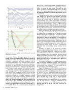
Fig. 9. (a) SW06 time-series at 14 phones, (b) PDFs for D (black), SR (red) and BR (green) paths at the 14 phones.
of sequential Bayesian filtering in space, that is, across phones. Because Bayesian filters have the power to exploit the correlation of motion of a target from one space/time point to another, it is possible to estimate parameters such as arrival times more tightly when we exploit spatial informa- tion rather than by only employing data at a single phone. Specifically, our signal arrives at a set of receivers via multi- ple paths and the movement of each arrival up and down the array of receivers can be compared to the motion of a target.
Figure 7(a) shows synthetic, noise-free time series at a tilted very large array (VLA) of 16 hydrophones in an isove- locity shallow water waveguide, similar to that of the Haro Strait Primer experiment.39 The hydrophones have varying, nonuniform vertical and horizontal separations, causing nonlinearities in the arrival time patterns. The direct (D) and surface reflection (SR) paths that sound follows can be iden- tified in the time series, although the SR is not present at the last two phones. Black dotted lines in the figure indicate the evolution of arrival times in space for each path. If we have a reliable arrival time estimate for one path at hydrophone k−1, we should be able to get an estimate for the same path at
12 Acoustics Today, July 2011
phone k, that is superior to an estimate obtained without tak- ing into account arrival times at neighboring receivers. Figure 7(b) shows the same signals after noise has been added. The Signal-to-Noise Ratio (SNR) was 14 dB. Red ellipses show spurious peaks introduced by noise that could be potentially identified by an arrival time estimator as true sound arrivals.
Treating each path in space as a moving target, Bayesian
MBP exploits the spatial evolution described above and
shown in Fig. 7(a). The state vector consists of the arrival
times for the D and SR paths. An observation model relates
the received time series to those state variables. A prediction
model is also selected, that predicts arrival times at receiver k
using arrival time knowledge at receiver k−1. Because of the
non-linearity of the observation model, KFs are not suitable
for this problem. Instead, MBP is implemented with particle
26
Figure 8(a) illustrates the true arrival times (+) and the corresponding estimates (o) for the 16 phones obtained via PF. Estimates are very close to the true arrivals with small deviations because of the added noise. Although two arrivals are detected for K=1,...,14, the filter correctly switches to a single arrival at phones 15 and 16. Figure 8(b) shows the PDF for the estimated number of arrivals at phone 14, where the PF clearly identifies two arrivals with probability of one. At phone 15, the PDF in Fig. 8(c) demonstrates that the filter has estimated the presence of a single arrival. Because of the tran- sition between phones 14 and 15, there is still significant probability (0.4) corresponding to the presence of two arrivals.
Similarly,27 we applied the PF arrival time estimation approach to data from the Shallow Water 06 (SW06) experi-
41
We consider three paths: D, SR, and Bottom Reflection (BR). As discussed,42 estimating accurately those arrivals can reduce uncertainty in source localization and subsequently, in inversion for other parameters. The state variables for the PF are the arrival times for the three paths.
Figure 9(b) demonstrates the PDFs of arrival times as calculated by the PF. Notable uncertainty is present at the 16th phone, as the PDF spread demonstrates. This is expect- ed, because no prior information from previous states (phones) is available; the 14th phone is where the PF begins. However, although the D and SR arrivals are very close at that phone, the PDFs show that the paths are clearly identified. The uncertainty is reduced at lower phones, where estimates are improved because of the incorporation of prior informa- tion. As also discussed,41 uncertainty, manifested by an increase in the spread of the PDFs, becomes more pro- nounced when the SR and BR paths cross at receivers six through three.
We consider here, as an additional state variable, the number of arrivals that are present in the time series.
filtering.
The data were collected in August 2006 at the 16-ele- ment MPL-VLA1 array. The source signal was a linear fre- quency modulated pulse with frequencies between 100 and 900 Hz; the sampling rate was 50 kHz. Received data were match-filtered to produce the time series of Fig. 9(a). Because of low SNR at the 15th and 16th phones, data at only the 14 lower phones were used.
ment.