Page 42 - Acoustics Today

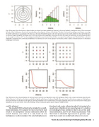
Fig. 4. Illustration of how the distances to detected objects can be used to estimate probability of detection for the case of randomly located point sensors. The area surveyed by bands of fixed width goes up linearly with increasing distance from the point, as shown in the left plot. Therefore, if we detected everything we would expect, on average, the number of detections to go up linearly with distance, as shown by the dashed histogram in the center plot. In practice, the number of detections drops off with distance, as shown by the green histogram. By fitting a curve to this (red solid line) and comparing it with a projection from the origin (red dashed line), we can estimate detectabil- ity: for example, at a distance of 2.2 we observed approximately half as many detections (blue solid line) as we expect if everything was seen (blue dashed line), so detection probability is estimated to be 0.5. Detection probabilities for all distances are shown in the right plot (red solid line), which is called a “detection function” in the distance sampling survey literature.
Fig. 5. Illustration of how the spatial pattern of a detected sound (red circles) on a hypothetical array of 16 hydrophones (black circles) contains information about the prob- ability of detection. In the left case, the detection probability is high for small distances, but drops off rapidly. Hence each sound is only heard on a compact set of hydrophones, but tends to be heard on all of them. In the right case, detection probability is low at small distances, but drops off gradually. Here, each sound is heard over widely spaced hydrophones, but not at all of them. This kind of thinking is the basis for spatially explicit capture recapture (SECR) methods.
directional, and so give information about the bearing to the sound source. Members of our research group at St. Andrews are extending the basic method so that it can use this addi- tional information, and we have found in preliminary work that it leads to substantial improvements in precision, espe- cially when sounds are usually heard only on few sensors.
could be obtained.
The standard SECR method can be extended to use addi-
tional information. For example, the time of arrival of each sound at the hydrophones contains information about the sound’s location, even when it is only heard on two hydrophones. Another example is that some hydrophones are
Passive Acoustic Monitoring for Estimating Animal Density 41