Page 40 - Acoustics Today

extent, cue rate—implying tagging more whales. As we have discussed, performing the tagging study during the main sur- vey would also be better.
Examples of other ways to estimate detectability
We presented our first example in some detail, to show the complexities that can be involved and the potential issues of which to beware, particularly with the multipliers. However, cue counting of echolocation clicks is not the only approach for obtaining a count, and using tagging data is not the only way to estimate detectability. Here, we illustrate the diversity of approaches with a few more examples. We start with methods that rely on having good acoustic data, in the sense of many hydrophones closely spaced and in some cases sophisticated acoustic processing. We end up with approaches that are more applicable in situations where data are sparser. In these latter cases, inferences will be correspondingly less reliable.
Total counts—beaked and sperm whales in the Bahamas
These two examples illustrate the case where we can assume that all objects within some defined spatial boundary are detected, and all outside that boundary can be excluded. Hence, we do not need to worry about false negatives. In both of these examples, the false positive rate is also negligible. Both examples are based on data from the 82-hydrophone bottom-mounted array at Tongue of the Ocean, Bahamas.
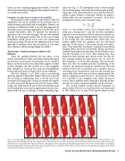
The first (Moretti et al., 2010) used a cue-counting approach applied to Blainville’s beaked whale, but instead of the cue being an echolocation click, it was the start of the vocal part of a foraging dive. Groups of animals dive togeth- er, and at some point during their descent they begin echolo- cating. The clicks produced can be detected relatively easily on the hydrophone array, and an approximate location deter- mined either by eye or through a simple smoothing algo-
rithm (see Fig. 3). The hydrophone array is dense enough that no diving groups can be missed; we also require that div- ing groups can be separated with accuracy, and that the local- ization is good enough to determine whether the group is diving within the area monitored or outside. Given these assumptions, density can be estimated using
(3)
where n is the number of dive starts recorded within the study area a during time T, and the two other multipliers required to convert density of dives to density of animals are 𝑔ˆ, the average group size (obtained from visual surveys) and
ˆ
𝑑, the average dive rate, obtained from DTAG data. The
authors applied both this approach and the click-based approach to data from a 3-day period during navy opera- tions. They found that the density of animals (undertaking foraging dives) decreased substantially during operations, compared with before and after them, but that’s another story (see also McCarthy et al., 2011). More relevant here, they found that both methods gave similar results, but that the dive counting method was more precise (CV of 11.9% for dive counting vs. 21.4% for click counting). This was because there were only two random quantities contributing to the variance—the estimates of group size and dive rate. Since the number of dive starts was assumed to be a complete count of everything in the surveyed area, and since the surveyed area covered the whole of the area we wish to estimate density for, then no randomness came from the n. The lesson here is that if it is possible to do a complete count within the area of interest, this is probably better, although it depends on how precisely the various required multipliers can be estimated.
The second example involves density estimation of sperm whales (Physeter macrocephalus) from a 42-day period in 2007 (Ward et al., in press 2012). Sperm whales are also
Fig. 3. A set of heatmaps showing the output of a smoothing algorithm applied to the number of Blainville’s beaked whale clicks detected at each of 82 hydrophones in the Tongue of the Ocean, Bahamas (cf. Fig. 1 for range location). White indicates the most clicks, then yellow, then red. Each plot includes 10 minutes of data, and successive plots advance by 1 minute from left to right, top to bottom. There appears to be one group diving at the beginning of the time series, at the center left (maybe a second group is present during the first 10 minutes, at the bottom, likely outside the range). A new dive starts (the “objects” counted in the dive counting method) to appear around minute 4, being clearly visible from around minutes 9 onwards.
Passive Acoustic Monitoring for Estimating Animal Density 39