Page 39 - Acoustics Today

whales show quite metronomic diving behavior (see discus- sion in Marques et al., 2009 paper). However, for other species and other contexts it may not be, given that vocaliza- tion rates can vary in marine mammals as a function of time of day, year, group size, season, bottom depth, location, etc. If the relationship between cue rate and these factors is known, it may be possible to use a modeling approach to predict mean cue rate during the time of the survey. For example, if cue rate depends on local group size then one would need an estimate of the relationship between cue rate and group size (from a statistical model), and also the distribution of group sizes during the survey period of interest. One important limitation arises when cue rate depends on animal density itself—in this case the only option is to measure it within the study area during the time period of interest.
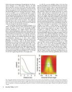
For estimating the detection probability, Marques et al. (2009) were able to match up clicks produced by the tagged whales with those received on the surrounding bottom- mounted hydrophones. The simplest analysis would have been to take all hydrophones within an 8 km radius of the whale and calculate what proportion of the emitted clicks was received. However, because there was a relatively small num- ber of dives (only 15 with tracks), and they did not wish to assume that animals were randomly distributed with respect to hydrophones, Marques et al. took a more complex approach. This involved building a regression model of the probability of detecting a click on the bottom-mounted hydrophones as a function of direct-path distance and hori- zontal and vertical angle of the whale with respect to the hydrophones. The angles were important because the echolo- cation clicks of beaked whales are highly directional. Given the fitted regression model (see Fig. 2), a Monte-Carlo pro- cedure was used to integrate out distance and angle, and yield an estimated average detection probability of 𝑝ˆ = 0.032 with CV of 15.9% (again using the dive as the sample unit).
As with the cue rate multiplier, there is the issue that detection probability was not estimated at the same time and place as the density dataset. There is a particular potential for bias here because tagging studies can only take place under calm sea conditions which may not be representative of aver- age conditions. Indeed, the average wind speed at a nearby weather station during the 6-day period of the survey was 12.4 kn, while the average speed when the tags were on was only 6.1 kn. Higher wind speed could reduce detectability, causing the estimate of detection probability using the tags to be too high. One option to address this would be to include wind speed in the detection probability regression model— however, predicting detectability at wind speeds observed in the 6-day period would then mean extrapolating outside the range of the data from the tag periods, so this approach is unlikely to be reliable. A second option is to analytically model the effect of increased noise on the detection algo- rithm. Instead, being empiricists, we chose a third option, described in a follow-up study (Ward et al., 2011), that involves measuring the effect. Ward et al. (2011) added noise from sound samples taken at the study area under a variety of wind speeds to the original hydrophone recordings, re-ran the detection algorithm, and determined the reduction in performance caused by the additional noise. They found that detection probability was indeed lower at higher noise levels, although not by as much as one would predict from theory.
Putting all of the above together, Marques et al. (2009) came up with a density estimate of 25.2 animals per 1000 km2, with a CV of 19.5% and corresponding confidence interval of 17.3-36.9. The estimate contains 4 random com- ponents: n (number of clicks), 𝑐ˆ (false positive rate), 𝑝ˆ (detec- tion probability) and 𝑟ˆ (cue rate). The percentage contribu- tion to the overall variance of these was, respectively, 8, 1, 66 and 25%. Hence, to reduce uncertainty, the thing to focus on in this study would be detection probability and, to a lesser
Fig. 2. Estimated probability of detecting a Blainville’s beaked whale echolocation click on bottom-mounted hydrophones at the Atlantic Undersea Testing and Evaluation Center (AUTEC), derived from a regression analysis on tagged whales at known locations and orientations relative to the hydrophones. The left plot shows probability of detection as a function of distance for clicks where the animal is pointed directly at the hydrophones (black line) and at off-axis angles of 45 and 70 degrees (green and blue lines). The right plot is a heatmap showing probability of detection as a function of vertical and horizontal off-axis angles, evaluated at the smallest observed distance (0.46km).
38 Acoustics Today, July 2012