Page 18 - Winter2014

from a numerical model or data. In terms of our soliton work, this is particularly useful, as solitons are a nonlinear phenomenon, and even the best model/data will show substantial enough changes in N, Δc, L and λ due to this effect. This is in addition to the normal fluctuation in the internal waves due to changing density stratifica- tion and currents. Seeing how big such fluctuations are, and how they affect useful acoustic quantities such as Lcoh is part of our ongoing research.
In the depth averaged approach to estimating Lcoh, simplifica-
tion was achieved by just considering the vertical average of the sound-speed perturbation. However, we can also use the simple perturbation theory forms to look at the detailed vertical sound- speed structure. This is most easily done in the acoustic normal mode picture, which happily is also a very good descriptor of low frequency, shallow water acoustics. The results obtained will now be on a mode-by-mode basis, i.e.; LcohLcoh(n) each mode now has its own coherence length. The perturbed phase accumulation over each modal path to the broadside array, ∆φn = ∫∆ Lcoh LCr can be expressed using a simple background waveguide (e.g. the “hard bot- tom” waveguide, with analytic eigenvalues)
which is perturbed by a mixed layer and internal waves below the mixed layer. In a simple “square wave soliton” approximation (Lynch et al., 2010), we can write the perturbed wavenumber as
In the above, all the parameters that comprise the wavenumbers are very simple environmental quantities, so that the physical depen- dence on the environment is very clear. Specifically, H1W is the internal wave peak depth, D is the mixed layer depth, H is the water
column depth, and n is an integer (the mode number). If we inte- grate the ∆k1W along the path, we get a very similar result to what
we had in the depth-averaged case, i.e.
The modal form is just as simple as the depth averaged form, and
now has the added richness of including the water column vertical
structure in the ∆k1W term. This form can also include bottom prop- n
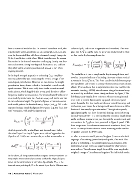
erty variability, and be used to compare bottom versus water column effects. We would note that in experiments where one can filter the modes in time (e.g. SW06), the coherence along a horizontal array on a mode by mode basis shows clearly, as shown by Figure 5. The left three panels visually show coherence when no strong internal wave train is present. Ignoring the top panel, the second panel
down shows the first four mode arrivals on a vertical line array, and the bottom panel shows the arriving modal wave-fronts on a 465m horizontal line array lying on the seabed. The right three panels, again ignoring the top, show the arrivals during a period of strong internal wave activity – it is obvious that the coherence length drops as the nonlinear internal waves pass through the acoustic track, and the numbers for Lcoh have been presented in Figure 3, panel 3. We have not pursued the coherence versus mode number in detail, but we do see the qualitative decrease versus increasing mode number we predict above in the SW06 data.
As a last note on the modal picture (See figure 5), we can also look at groups of interfering (unresolved) multipaths, if we wish. This pushes us to looking at the complex pressure, and makes a little more mess, but can be treated largely similarly to what we have shown above. The coherence length then will be some amplitude- weighted average of the coherence lengths of the individual modes.
n
16 | Acoustics Today | Winter 2014