Page 17 - Winter2014

Euclidean geometry in the horizontal direction and equally simple first order perturbation theory forms for the features when includ- ing their vertical structure. Beginning work on this using depth averaged ocean features was discussed in the Bill Carey memorial session of the UA in Corfu (Lynch et al, 2013), and showed the ba- sic equations for Lcoh for a number of the ocean features we listed, as well as numerical results for a shelf-break front (based on the SW06 region parameters). In this paper, we are extending that work to show numbers for the effects of nonlinear internal waves, so that we can cross compare two of the “major players” in creating acoustic field spatial decoherence. We will, given the limited space, stick to the simplest “depth averaged ocean” and “resolved modes” cases, and hope to eventually include the whole feature model story (interfer- ing modes and rays, and the many other ocean/seabed effects) in a future article.
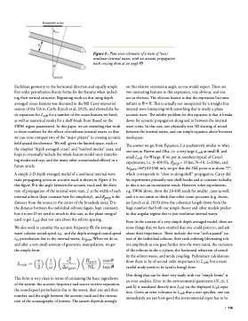
A simple 2-D depth averaged model of a nonlinear internal wave train propagating across an acoustic track is shown in Figure 4. In this figure, θ is the angle between the acoustic track and the direc- tion of propagation of the internal wave train, L is the width of each internal soliton (kept constant here for simplicity), and Rperp is the distance from the source to the center of the broadside array. D is the distance between the individual solitons (again, kept constant), but it is not D we need so much in this case, as the phase integral used to get Lcoh does not care about the soliton spacing.
We also need to consider the acoustic frequency π, the average water column sound-speed co, and the depth averaged sound-speed co perturbation due to the internal waves, ∆cpert. When we do so, and after a very small amount of geometric manipulation, we get the simple form:
This form is very clean in terms of containing the basic ingredients of the system: the acoustic frequency and source receiver separation, the sound-speed perturbation due to the waves, their size and their number, and the angle between the acoustic track and the orienta- tion of the oceanography of interest. The answer depends strongly
on this relative orientation angle, as one would expect. There are two interesting features to this expression, one obvious, and one
not as obvious. The obvious feature is that the expression becomes infinite at θ = 0. This is actually not unexpected for a straight line internal wave interacting with something that is nearly a plane acoustic wave. The subtler problem for this equation is that it breaks down for acoustic propagation along and in between the internal wave crests. In this case, one physically sees 3D ducting of sound between the internal waves, and our simple equation above becomes inadequate.
The answer we get from Equation 2 is qualitatively similar to what one sees in Finette and Oba, i.e. a very large Lcoh at small θ, and small Lcoh for θ large. If we put in numbers typical of Carey’s experiments, i.e. f= 400 Hz, Rperp = 10 km, N=10, L=200m, and ∆cpert.=40*(10/100) m/s, we get that the 30λ point is at about 77°, which corresponds to “close to along-shelf ” propagation. Carey did his experiments primarily near shelf-breaks and at constant isobaths, so this is not an inconsistent result. However, other experiments, e.g. SW06 above, show the 20-40λ result for smaller cases as well, and it is not amiss to think that other ocean processes (e.g. fronts, see Lynch et al, 2013) drive the coherence length down from the large number that both our simple theory and other models predict in that angular regime due to just nonlinear internal waves.
Even in the context of a very simple depth averaged model, there are some things that we have omitted that one could point to, and ask about their importance. These include: the true “sech squared” na- ture of the individual solitons, their rank ordering (decreasing soli- ton amplitude as one goes further into the wave train), the curvature of the solitons in the x-y plane, the horizontal refraction of sound
by the soliton waves, and mode coupling. Preliminary calculations show these to be of second order importance to Lcoh, but a more careful study needs to be (and is being) done.
One thing that can be done very easily with our “simple forms” is an error analysis. Error in the environmental parameters (N, Δc, L and λ) is translated directly into Lcoh via the displayed Lcoh equa- tion. Given an error tolerance in Lcoh that a user specifies, one can immediately see just how good the environmental input has to be
Figure 4 : Plan-view schematic of a train of (two) nonlinear internal waves, with an acoustic propagation track crossing them at an angle Θ.
| 15