Page 21 - Spring 2015

rics) measured from impact pile driving are on the order of 220 dB re 1 μPa at a range of ~10 m from 0.75-m-diameter piles (Reinhall and Dahl, 2011) and on the order of 200 dB re 1 μPa at a range of 300 m from piles that are 5 m in diam- eter (Lippert and von Estorff, 2014b). Loud impulsive un- derwater sounds can potentially have physiological effects on fish (Halvorsen et al., 2012a,b; Casper et al., 2013a,b) and on marine mammals (Southall et al., 2007; Lucke et al., 2009; Kastelein et al., 2015). At greater distances from the source or at lower sound levels, the potential effects include mask- ing of biologically important sounds and/or the effects on behavior (Southall et al., 2007; Popper et al., 2014). There- fore, both environmental monitoring and noise mitigation efforts invariably accompany impact pile driving particu- larly in biologically sensitive underwater habitats.
The Predominant High-Pressure
Underwater noise field
There is both theoretical consensus and experimental evi-
dence that the predominant high-pressure underwater noise
field from impact pile driving on hollow steel piles can be
attributed to a “Mach wave” effect (Reinhall and Dahl, 2011;
Dahl and Reinhall 2013; Zampolli, et al., 2013; Lippert and
von Estorff, 2014a). This effect arises from a rapidly moving
sound source generated by a deformation of the pile wall that
is traveling down the pile on hammer impact. This deforma-
tion, or bulge, is the consequence of the Poisson effect where
a material compressed in one direction (here vertically by
hammer impact) expands in another direction, in this case
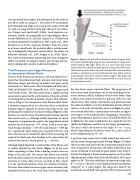
producing the momentary outward swelling (Figure 2) that
behaves as a sound source. The downward traveling speed of
Figure 2. Bulge in the pile wall (red lines) as result of impact ham- mer strike (symbolized by large arrow) and subsequent compression of pile material. The bulge, which acts as a source of sound, travels successively down the pile at speed cs and at L/cs s later (blue line). Wave fronts from the earlier emission (red) and later emission (blue) are shown with all prior emissions (black lines); they add up to form a quasi-planar wave front characterized by angle θ. This angle and the associated time delays can be measured with a vertical array of 9 hydrophones (circles).
the later lower source emission (blue). The progression of wave fronts from all positions up to and including the lat- est are shown in black. Addition of these wave fronts form a Mach cone centered around the pile axis (only one side shown here). This simple construction also illustrates how the coherent addition of a line distribution of time-delayed sources, such as the red and blue sources in Figure 2, gener-
this sound source, cs, although mildly dependent on sound
In-Line Symbols and Equations (Dahl, de Jong and Popper article)
in Figure 2), this array would d#e2tect the sou𝐿𝐿n/𝑐𝑐d! first on the speed of the stee#l1material, 𝑌𝑌/𝜌𝜌 , where Y and ρ are the ma- shallow hydrophones and later on the deeper hydrophones.
frequency, is approximately equal to the longitudinal sound
terial Young’s modulus (~ 200 GPa) and density (~7,850 kg/ !! !w/!s
#2 𝐿𝐿/𝑐𝑐!
m3), respectively. These values put cs equal to 5,0I5n0-Lmin/se, Saynmd bols and Equations (Dahl, de Jong and Popper awrticle) s
in the neighborhood of 15 - 19°. this value that can be indirectly o!b!served by measuring the #4
15 − 19°
#1 𝑌𝑌/𝜌𝜌
A pressure-time series versus depth taken from such verti-
, ~1,500 m/s.
Although highly idealized, a notional idea of the Mach cone
# 6 and # 7 𝑅𝑅∗
bulge in the pile wall. The source that moves successively
#4
#3 𝜃𝜃=sin 𝑐𝑐!/𝑐𝑐!
angle of the Mach cone that develops in the water where the
sound waves travel at sound speed, c #4 15−19° w
𝐿𝐿c/al𝑐𝑐 line array during impact pile driving (Figure 3) clearly !
∗
#5 𝑅𝑅 =𝐻𝐻/tan𝜃𝜃
shows the expected delay with the measurement depth of the
very strong arrival (first peak in#th6eanyedl#lo7w sh𝑅𝑅aded area) that !!
is readily obtained by the sketch (Figure 2) of the wave #3
𝜃𝜃=sin 𝑐𝑐!/𝑐𝑐!
∗
fronts expanding in time from a moving sound source or
can be attributed to the kind of quasi-planar wave front il- lustrated in Figure 2. Beam-forming analysis on the yellow
down the pile is shown in two arbitrary positions: first in red
shaded portion of these data (Dahl and Reinhall, 2013) gives
#8 /𝑅𝑅∗
and then at a time delay L/cs (in seconds) in blue, where
angle θ as 18°. This also establishes an important range scale,
L is the separation between these two arbitrary positions. #9 1/𝑇𝑇
#9 1/𝑇𝑇
𝑅𝑅R* = 𝐻𝐻/tan 𝜃𝜃 , where H is water depth at the pile installation,
The wave fronts from the earlier upper source emission (red) expanded farther out in the water than those emitted from
setting R* to ~3 water depths. For ranges less than R* the #10 𝑝𝑝 !"#
#6and#7 #11 (𝑝𝑝!"# 𝑝𝑝ref) #8
un∗derwater sound field varies greatly with the measurement 𝑅𝑅
#10 𝑝𝑝 !"#
#2
∗
#5 𝑅𝑅 =𝐻𝐻/tan𝜃𝜃
#5
ates a sound field with a quasi-planar wave front at angle θ
with respect to the horizontal line. Imagining a vertical line
#1 𝑌𝑌/𝜌𝜌
array of hydrophones placed in such a sound field (black dot
The array could also measure#3the angle, 𝜃𝜃 = sin 𝑐𝑐c /𝑐𝑐c , which, depending on the precise values of c and c puts θ
15−19° ∗
#8 /𝑅𝑅∗
/𝑅𝑅∗
In-Line Symbols and Equations (Dahl, d
#11 ( 𝑝𝑝 !"# 𝑝𝑝ref)| 19
e