Page 47 - Spring 2015

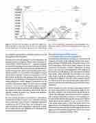
Figure 1. Schematic of the atmospheric boundary layer (ABL) show- ing the atmospheric surface layer (ASL; between the straight dashed line and the ground), mixed layer, capping inversion (curvy dashed
the complexity and predictive challenges inherent to sound propagation in the atmosphere.
The variability of sound propagation in the atmosphere has actually long been recognized. King (1919; see also the ac- count by Beyer [1999]) refers to the “...capricious behavior of sound-waves propagated in the open atmosphere [which] has been attributed to the existence of innumerable disconti- nuities of temperature, density and humidity, and to refrac- tion by gradients of wind-velocity.” Recordings by Ingard (1953) showed random variations in sound levels of 10-20 dB, which he attributed to the gustiness of the wind. Recent advances in the simulation of atmospheric turbulence and sound propagation enable dramatic visualizations of the variability identified by Ingard. [To view visual recordings visit: http://wp.me/p4zu0b-Qq]. Modern long-term experi- mental studies further demonstrate the challenge of predict- ing sound levels from atmospheric observations that are typically available in practice (e.g., Konishi and Maekawa, 2001; Valente et al., 2012).
The next section provides an introduction to atmospheric stratification and how it relates to the refraction of sound. Then we illustrate, using data from a nighttime experiment conducted on the US Great Plains, the challenge of accu- rately predicting sound propagation. Subsequent sections discuss representation and sampling of the atmosphere for sound propagation predictions.
line), and free troposphere. Near-ground sound propagation for a high-wind condition, with the wind blowing from left to right, is de- picted.
stratification and Refraction
in the near-Ground Atmosphere Environmental phenomena occurring over a broad span of temporal and spatial scales influence sound waves propa- gating outdoors. Turbulent eddies and gravity waves in the lower atmosphere, which scatter sound, range in size from centimeters to kilometers. Weather phenomena on much larger scales also impact the propagation. The emphasis of this article is on propagation in the atmospheric boundary layer (ABL), more specifically the lowermost 10% of the ABL, which is called the atmospheric surface layer (ASL), as depicted in Figure 1. The ABL, which responds directly to surface processes on a diurnal timescale, is generally be- tween 0.5 and 3 km deep depending on latitude and weather conditions.
When variations in terrain elevation and ground properties are weak, mean gradients of the atmospheric fields are usu- ally much stronger in the vertical than in the horizontal di- rection. The atmosphere may then be described as horizon- tally stratified. Refraction of sound in such conditions can be most readily understood using the concept of an effective sound speed, which is defined as ceff = c+u cos θ, where c is the actual sound speed, u is the wind speed, and θ is the angle between the azimuthal direction of propagation and the wind vector. The sound speed itself is proportional to the square root of the absolute temperature; there is also a weak dependence on humidity (Ostashev, 1997).
| 45