Page 49 - Spring 2015

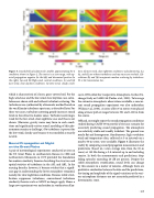
Figure 3. Sound-field calculations for profiles approximating the 4 conditions shown in Figure 2. The source is at zero range, with up- wind propagation negative (to the left) and downwind positive (to the right). (a) and (b) High-wind, neutral conditions. (c) and (d) Low-wind, clear daytime conditions. (e) Zero-wind, cloudy condi-
which is characteristic of a loose, grass-covered soil. For the high-wind case and the low-wind, clear daytime case, calcu- lations are shown with and without turbulent scattering. The turbulence was synthesized by a kinematic method based on the von Kármán turbulence spectrum, as described later. For these two cases, turbulent scattering greatly increases sound levels in the refractive shadow zones. Turbulent scattering is weak for the low-wind, clear nighttime case and thus is not shown. (However, gravity waves may form in such condi- tions and significantly scatter sound; modeling of this phe- nomenon remains a challenge.) No turbulence is present for the low-wind, cloudy case because it was modeled as exactly neutral.
sound Propagation at night
on the Great Plains
A pair of meteorological experiments conducted at sites on the US Great Plains in southwestern Kansas in 1968 and northwestern Minnesota in 1973 provided the foundation for modern similarity theories describing the structure and spatial statistics of turbulence in the ASL and ABL. In the ensuing decades, however, it became evident that a signifi- cant gap in understanding the lower atmosphere remained, namely, for clear nighttime conditions. Because stable strati- fication suppresses turbulence, conventional turbulence similarity theories such as MOST no longer apply. Hence a large new experiment was undertaken in southeastern Kan-
tions. (f) Low-wind, clear nighttime conditions. Calculations (a), (c), (e), and (f) are without turbulence and ray traces are overlaid. Cal- culations (b) and (d) incorporate random scattering by turbulence. TL is the transmission loss.
sas in 1999 called the Cooperative Atmosphere–Surface Ex- change Study or CASES-99 (Poulos et al., 2002). To leverage the extensive atmospheric observations available, a concur- rent sound propagation experiment was also undertaken (Wilson et al., 2003). A series of five 6-m towers were placed along a linear path at ranges between 361 and 1,180 m from the source.
Offhand, one might expect the sound propagation conditions studied during CASES-99 to provide a best case scenario for accurately predicting sound propagation. The atmosphere was relatively stable and weakly turbulent. The ground was nearly flat and homogenous. Simultaneous, high-resolution wind and temperature data, collected at 5-m intervals on a nearby 60-m tower, were available. Figure 4 illustrates the reality by comparing sound propagation measurements and predictions (based on 1-min average data from the 60-m tower) at 150 Hz during a 2-h interval up to and including sunrise. In both the measurements and predictions, deep fading episodes exceeding 20 dB are present. Despite the stable atmospheric stratification, sound levels can change by this amount in a matter of minutes. Although there are qualitative similarities between the data and the predictions, the timing and amplitude of the signal variations at the vari- ous microphone distances are not accurately predicted in a deterministic sense.
| 47