Page 50 - Spring 2015

sound Propagation in the Atmospheric boundary layer
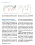
Figure 4. Sound propagation measurements (left) and predictions (right) at 150 Hz during CASES-99 intensive observation period 7 (October 18, 1999). Shown are 3 different ranges from the source: 570
Representation of the Atmosphere
As illustrated by CASES-99, the atmosphere possesses a complex spatial and temporal structure that impacts sound waves strongly. Realistic high-resolution representation of the ABL is a particularly important and challenging aspect of simulating wave propagation in the atmosphere. One ap- proach is to employ computational fluid dynamics (CFD) simulations of the atmosphere and turbulence as input to the sound propagation calculations. Among the various classes of CFD, large-eddy simulation (LES) generally best cap- tures the dynamics of turbulence in the ABL (Galperin and Orszag, 1993). The main drawbacks of LES are its computa- tional intensiveness (which may, in practice, far exceed the sound propagation calculation) and its resolution (which is typically no better than a few meters and thus most suitable for sound propagation at low frequencies). Besides LES, me- soscale numerical weather prediction (NWP) models can be employed (Lihoreau et al., 2006). Ordinary mesoscale mod- els do not simulate turbulence and generally have a much lower resolution than LES. However, they are particularly useful for simulating flows in terrain with varying elevation and land surface properties.
Turbulence can also be synthesized with kinematic ap- proaches, meaning that the fields are synthesized from pre- scribed spatial statistics, rather than by attempting to solve fluid-dynamic equations. Relative to CFD, the main advan- tages of the kinematic approaches are their efficiency, high resolution, and simplicity. Kinematic approaches have been
m (blue), 760 m (green), and 1,170 m (red). Universal Coordinated Time (UTC) at the site precedes local standard time by 5 h. Reprinted from Wilson et al. (2003).
commonly used in acoustical modeling since the 1990s (e.g., Gilbert et al., 1990). The lack of realistic dynamics may not be important for calculating second-order statistics of the scattered sound field, such as the mean square sound pres- sure. Most kinematic approaches involve spectral synthesis from a superposition of spatial Fourier modes (harmonic functions). The amplitudes of the modes are made propor- tional to the square root of the spectral density at that wave number, whereas the phases of the modes are independently randomized. Application of an inverse transform (from the wave number to the spatial domain) then yields a random field consistent with the desired spectrum. An alternative to the spectrally based methods, but nonetheless a kinematic method, involves representing the turbulence field as a col- lection of randomly positioned, eddylike structures (Goede- cke et al., 2004).
The kinematic spectral methods as well as theories for wave propagation through turbulence require a model spatial spectrum for the turbulence. Although Gaussian spectral models have often been used in outdoor sound propaga- tion, the Kolmogorov or von Kármán spectrum are more realistic (e.g., Ostashev, 1997). MOST and other turbulence similarity theories can be useful for predicting parameters in the turbulence spectra from available atmospheric mea- surements. The CNPE calculations shown in Figure 3,b and d, incorporated turbulent scattering based on single realiza- tions of a von Kármán spectrum with height-dependent pa- rameters, as detailed by Wilson et al. (2008).
48 | Acoustics Today | Spring 2015