Page 51 - Spring 2015

sampling of the Atmosphere
Rarely, if ever, are measurements of the atmosphere and ter- rain available with the subwavelength resolution necessary to accurately predict the sound field in a deterministic sense (e.g., Wilson et al., 2008; Gauvreau, 2013), thus hindering validation of computational models. This motivates a num- ber of important practical questions regarding the use of meteorological data in outdoor sound propagation predic- tions. What types of meteorological data are most suitable, i.e., data from a vertical tower, weather balloons, weather radar or LIDAR, or a numerical weather prediction (NWP) model? How should the data be averaged and otherwise pro- cessed before usage in acoustic models?
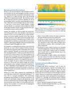
Suppose, for example, we wish to predict the sound expo- sure level associated with a short-duration event such as an explosion. It may seem reasonable to use a single instanta- neous set of vertical profiles recorded at the same time as the event. However, such profiles include the random turbu- lence present at the time of the observation. In effect, one is assuming that the turbulence extends infinitely in a horizon- tal plane, as illustrated in Figure 5. This has been aptly called a “plywood” model (Wyngaard et al., 2001).
For simplicity, we distinguish here between event and mean prediction. An event is short compared with the timescale over which the propagation effects decorrelate due to atmo- spheric variations. Examples are sound from an explosion and sound produced by a steady source but observed over an interval of several seconds or less. Mean predictions, in practice, refer to an average over a time interval long enough to remove the variability associated with individual events. In the atmospheric sciences, it is recognized that time in- tervals of roughly 30 min or longer are needed for good estimates of means and even longer averages for second- order statistics such as variances and spectra (Lenschow et al., 1994). Regarding sound propagation, spatial averaging along the propagation path and the frequency diversity in broadband signals may possibly mitigate the need for such long averaging times.
Wilson et al. (2007, 2008) examined the predictability of event and mean sound levels using high-resolution (1- to 4-m) LES as a surrogate atmosphere. After numerically propagating sound through the turbulence simulations, the results were statistically compared with predictions based on lower resolution but more typically available atmospheric characterizations such as mean vertical profiles and instan- taneous vertical profiles at a location near the propagation path. The main conclusions were:
Figure 5. (Top) Example of a realization of a turbulent velocity field (fluctuations plus mean vertical profile) in a vertical plane. (Bottom) Plywood model based on extending the fluctuations at a single range to the entire domain.
1. Mean vertical profiles produce the most accurate pre- dictions of both mean and event sound levels.
2. Predictions of mean sound levels from mean vertical profiles have relatively low root-mean-square (rms) er- rors, typically less than 2 dB, except in shadow zones and interference minima, where scattering by turbu- lence is important.
3. Predictions of mean sound levels based on averaging individual propagation calculations from many instan- taneous vertical profile samples results in overpredic- tion of sound levels in upward refraction due to the plywood atmosphere effect.
4. Event propagation is highly random and predictions have rms errors of 8-10 dB, even when they are based on local vertical profile data synchronized to the time of the propagation event.
Incorporating and Quantifying Uncertainty
In complex high-fidelity simulations, such as those for outdoor sound propagation, imperfect knowledge leads to errors at many stages of the modeling process. The error budget cannot be uniquely specified or computed exactly because the sources of error are not always known or quan- tifiable. However, an agreed-upon framework for the error budget can provide a useful starting point for describing un- certainties in a thorough self-consistent manner. Ghanem (2005) suggested the following hierarchical decomposition of modeling errors:
1. Errors reducible through better physics models.
2. Errors reducible through better data, e.g., more accu-
rate and precise measurements.
| 49