Page 53 - Spring 2015

tervals, where N is the number of samples to be drawn. A grid consists of NM cubes, where M is the number of random variables. One sample is then randomly drawn from each row and each column in the grid so that each interval of a variable is sampled once.
Variables that would not normally be considered stochastic, such as frequency, can be incorporated into the Monte Carlo integration. This approach provides a substantial computa- tional benefit: one can simultaneously sample over frequen- cy and the uncertain variables (Wilson et al., 2014). LHS can be particularly useful in assuring that some parts of the fre- quency spectrum do not go undersampled. For example, the strata can coincide with octave or one-third octave bands. Temporal integrations (over time of day or season) can be handled by the same approach.
Let us consider a numerical example illustrating the impacts
of uncertainty. The model atmosphere is neutrally stratified,
and refraction and scattering by turbulence are included in
the calculations using a CNPE and kinematic turbulence re-
alizations. The vertical profiles and turbulence spectrum are
modeled with MOST. The source is harmonic, with a fre-
quency of 100 Hz. To represent uncertainty in the environ-
mental state, six model parameters are assumed to be ran-
domly distributed: source height, ground porosity, ground
static flow resistivity, ground roughness, friction velocity,
and wind direction. Because the first five of these param-
eters are positive definite, they are modeled with log-normal
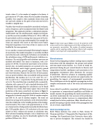
Figure 6. Root-mean-square (RMS) errors for the prediction of the mean sound level at a single frequency (100 Hz) resulting from vari- ous parametric uncertainties. The number of random parameter samples and the sampling method (ordinary Monte Carlo sampling [MCS] or Latin hypercube sampling [LHS]) were varied.
Conclusions
Sound waves propagating outdoors undergo many complex
interactions with the atmosphere, the ground, and natural
and man-made terrain features. As a result of steady im-
provement during the past several decades in theories and
computational models, randomness and uncertainty in the
propagation environment often determine the accuracy
of predictions. However, advances in computing capabili-
ties and MCS methods also provide new opportunities for
quantifying the impacts of environmental uncertainties.
These techniques can also be applied to propagation in other
complex environments such as the ocean and architectural
distributions. The medians are 5 m, 0.27, 2x10-6 Pa s m-2 ,
In-line Equations and Symbols
0.01 m, and 0.6 m s-1, respectively; the log deviations are all
!
set to10.𝑅𝑅4. The wind direction is modeled with a normal dis-
tribution, with a mean of 0° and a standard deviation of 40°.
! !" 𝑅𝑅 64 =2.8s×p1a0ces.
Additional details regarding the calculations can be found in Wilson et al. (2014). Root-mean-square (rms) errors for
Issues related to predictive uncertainty will likely increase
𝑐𝑐 =𝑐𝑐+𝑢𝑢cos𝜃𝜃 𝑁𝑁!
prediction of the mean sound level are shown in Figure 6.
eff
in importance as computational capabilities and fidelity of !! mode!ls! improve. By quantifying the model sensitivities, we
Shown are upwind and downwind predictions in which the
𝑢𝑢 2×10 Pasm
integrand is evaluated using MCS (with 16 random samples) and LHS (8, 16, and 32 random samples). The errors are
can better understand the true accuracy of the predictions −0.0098° and determine whether increases in computational effort about twice as large in the upwind as in the downwind0.d6irmecs-!! actually lead to better predictions. Effort should not be ex-
tion; t𝑢𝑢hi;s is likely due to the variable position of the shadow-
∗ pended attempting to predict details of the propagation that
are, in essence, unpredictable.
Acknowledgments
Keith Wilson dedicates this article to Profs. Dennis W. Thomson and John C. Wyngaard of the Department of Me- teorology, The Pennsylvania State University, whose influ-
zone boundary. The errors scale approximately as 1/ 𝑁𝑁, (𝑄𝑄 )
as is cha!racteristic of independent normally distributed sam-
ples. LHS provides about a 25% reduction in the rms error
(𝑧𝑧)
relative to MCS, without any increase in calculation time.
More advanced sampling strategies, such as importance and
(𝛽𝛽=𝑔𝑔 𝑇𝑇; !
adaptive sampling, can also be beneficially applied to this problem (Wilson et al., 2014).
𝑔𝑔 ence is present throughout. This research was funded by
𝑇𝑇!
𝑢𝑢∗ = 0.6
| 51