Page 58 - Spring 2015

objective bayesian Analysis in Acoustics
ing the realization observed as a function of the parameter Θ. It is often called the likelihood function. This likelihood represents the probability of fitting the measured data D to the hypothesis realized by the parameter Θ via model H(Θ). A straightforward way to quantify this fitting is to build a difference function between the modeled realization H(Θ) and the experimental data D. The difference function is also called residual error. In other words, the likelihood function is simply the probability of the residual error.
The term p(Θ|D) represents the probability of parameter Θ given the data D after taking the data into account. It is therefore called the posterior probability. The quantity p(D) on the left-hand side of Equation 2 represents the probabil- ity that the data are observed. After the data measurement, it is a normalization constant and ensures that the posterior probability (density function) integrates to unity.
Figure 2. Model-based parameter estimation scheme is an inverse problem. Based on a set of experimental data and a model (hy- pothesis), the task is to estimate the parameters encapsulated in the model. In general, the experimenter knows that an appropriate set of parameters will generate a hypothesized “data” realization that ap- proximates the experimental data.
Acousticians typically face data analysis tasks from experi- mental observations, and they are challenged to estimate a set of parameters encapsulated in the model H(Θ), also called the hypothesis. Figure 2 shows this task schemati- cally. The relevant background information is that the ex- perimenter knows that an appropriate set of parameters will generate a hypothesized “data” realization via a well-estab- lished prediction model (hypothesis) that approximates the experimental data well.
Figure 3 interprets Bayes’ theorem as presented in Equa- tion 2. The posterior probability, up to a normalization con- stant, p(D), is calculated by updating the prior probability, p(Θ). Once the experimental data D become available, the likelihood function p(D|Θ) is a multiplicative factor that modifies the prior probability so as to become the posterior probability (up to a normalization constant). Bayes’ theorem
56 | Acoustics Today | Spring 2015
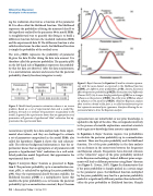
Figure 3. Bayes’ theorem (in Equation 2) used to estimate a param- eter with the same dataset as expressed in the likelihood function p(D|Θ), yet different prior probabilities [p(Θ); density functions] affect the posterior probability [p(Θ|D); density function] differently (Cowan 2007). (a) A more sharply peaked prior p(Θ) has a stronger influence on the posterior p(Θ|D). (b) A flat prior p(Θ) has almost no influence on the posterior p(Θ|D). Objective Bayesian analysis often involves a broad or flat prior, a so-called noninformative prior that represents maximal prior ignorance, therefore allowing the ex- perimental data to drive the Bayesian analysis.
represents how our initial belief, or our prior knowledge, is updated in the light of the data. This corresponds intuitively to the process of scientific exploration: acoustical scientists seek to gain new knowledge from acoustic experiments.
In Equation 2, Bayes’ theorem requires two probabilities to calculate the posterior probability up to a normalization constant. These are the prior probability and the likelihood function. Use of the prior probability in the data analysis was an element in the controversy between the frequentist and Bayesian schools. Frequentists have directed criticism at the “subjective” aspect of the prior probability involved in the Bayesian methodology. Indeed, different prior assign- ments will lead to different posteriors using Bayes’ theorem (see Figure 3; Cowan, 2007). Figure 3a demonstrates that if the prior probability is sharply peaked in a certain range in the parameter space, the likelihood function multiplied by the prior probability may lead to a posterior probability peaked at a significantly different position than indicated by either the prior probability or likelihood function. Sharply