Page 60 - Spring 2015

objective bayesian Analysis in Acoustics
(Gregory, 2010). To be precise, this Gaussian assignment is different from assuming the statistics of the residual errors to be Gaussian. It is the consequence of little information on the finite, yet unspecified, residual error variance being available.
In some other data analysis tasks, the experimenter knows only that the model represents the data well enough for the residual errors to have a noninfinite mean value. Taking ac- count of this finite mean in the maximum entropy proce- dure gives rise to an exponential distribution; in this case, the parameter space must not be unbounded above and below. (When the mean and variance are both noninfinite, the result is a Gaussian distribution with nonzero mean and finite variance.)
In summary, maximization of the Shannon-Jaynes entropy (Gregory, 2010) is a wholly objective procedure in the data analysis. The resulting distribution is guaranteed to show no bias for which there is no prior evidence.
Two levels of bayesian Inference
In many acoustic experiments, there are a finite number of
competing models (hypotheses), H1,H2,...,HM, that are in
competition to explain the data. In the room-acoustic ex-
ample above, H is specified in Equation 1 as containing one 1
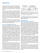
exponential decay term and one noise term, but the same data in Figure 1 may also be alternatively described by H2 containing two exponential decay terms (double-rate de- cay) with two further parameters. Only one of the models is expected to explain the data well. Figure 4 illustrates this scenario. In practice, architectural acousticians often expect single-, double-, or triple-rate energy decays (Xiang et al., 2011; Jasa and Xiang, 2012). In the case of plausible compet- ing models (e.g., double rate, triple rate), it would be un- helpful to apply an inappropriate model to the parameter estimation problem (Xiang et al., 2011). Before undertak- ing parameter estimation, one should ask, “Given the ex- perimental data and alternative models, which model is pre- ferred by the data?”
Bayesian data analysis applied to solving parameter esti- mation problems, as in the example above, is referred to as the first level of inference, whereas solving model selection problems is known as the second level of inference. Bayes- ian data analysis is capable of performing both the param- eter estimation and the model selection by use of Bayes’ theorem. We begin below with the second level of inference, namely model selection. This top-down approach is logical;
Figure 4. Second level of inference, model selection, is an inverse problem about selecting one of a finite set of models. Based on the experimental data and a finite set of models (hypotheses), the task is to infer which model is preferred by the data.
one should determine which of the competing models is ap- propriate before the parameters appearing in the model are estimated (Xiang, 2015).
Model selection:
The second level of Inference
Within a set of competing models, the more complex mod-
els (generally those with more estimable parameters) will al-
ways fit the data better. But models with excessive numbers
of parameters often generalize poorly (Jefferys and Berger,
1992). To penalize overparameterization, Bayes’ theorem
is, accordingly, applied to one of the competing models, HS,
among a finite model set, H1,H2,...,HM, , given the data D,
deferring any interest in model parameter values. We simply
of Bayes’ theorem, the likelihood function, p(D| HS) , is re- ferred to as the (Bayesian) evidence. The posterior probabil- ity of the model HS given the data D is simply proportional to the evidence because the principle of maximum entropy assigns identical prior probability to each model.
Although more complex models may fit the data better, they pay a penalty by strewing some of the prior probability for their parameters where the data subsequently indicate that those parameters are extremely unlikely to be. There is, therefore, a trade-off between goodness of fit and simplic- ity of model, and this can be seen as a quantitative general- ization of the qualitative principle known as Occam’s razor, which is to prefer the simpler theory that fits the facts (Jef- ferys and Berger, 1992).
The model selection process calculates the posterior prob- ability of each of the finite number of models to determine which model has the greatest posterior probability (or after an increasing trend, no more significant increases will be ob- served; Jeffreys, 1965) and, if desired, to rank the competing models.
58 | Acoustics Today | Spring 2015
replace Θ in Equation 2 by the model H . In this application S