Page 61 - Spring 2015

Parameter estimation:
The first level of Inference
Once a model has been selected according to the experimen-
tal data, denoted as model HS, then the Bayesian framework
is available to estimate its parameters ΘS. We now write the
model with its parameters explicit as HS(ΘS); for instance,
model H1(Θ1) in Equation 1 contains one exponential decay
term wFigthurietsEQpaUrAaTmIOetNeSrs collectively denoted as Θ1= {θ0, θ1,
θ2}. Bayes’ theorem is now applied as before so as to esti-
mate the parameters ΘS, given the model HS and the data D.
The quantity p(D) in E−θqut ation 2 now becomes p(D| H ), the H(Θ)=θ0 +θ1e 2 (1) S
probability of the data D given the model HS.
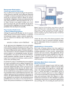
Figure 5. Stage house of opera/theatre venues features a stage shell (concert hall shaper) that is readily deployable to convert the opera/ ballet setting to symphonic performance setting (Jaffe, 2010). For symphonic purposes, the stage shell features acoustic coupling be- tween the reverberant stage house behind and above the shell with the main audience floor.
estimate the mean values of the relevant parameters, their uncertainties in terms of associated individual variances, and the relationships between the parameters of interest (Xiang, 2015).
Applications in Acoustics
Both levels of Bayesian inference have been applied in acoustics. This section briefly sets out some recent examples including applications in room acoustics, communication acoustics, and ocean acoustics. These applications all have in common the existence of well-established, or at least well- understood, models for predicting the processes under in- vestigation, yet only a set of experimental data is available to study the process.
Multiple-Rate Room-Acoustic
Decay Analysis
A number of recently designed concert halls have imple- mented reverberation chambers coupled to the main floor so as to create multiple-rate energy decays. A further appli- cation is the design and adaptation of a stage shell system, that is, a “concert hall shaper” in opera/theatre venues to couple with reverberant stage houses as shown in Figure 5 so as to attain two desirable yet competing auditory features: clarity and reverberance (Jaffe, 2010; Xiang et al., 2011). Architectural acousticians are often challenged to quantify reverberation characteristics in (connected) coupled spaces (Jasa and Xiang, 2012). On extending the model used in the
Two levels of Inference
in one Unified framework
Although the quantity p(D| HS) plays the role of a normal- izationpc(Θon|sDta)npt(Dat) t=hep(fiDrs|tΘle) vpe(Θl o)f. inference, it is(2id) entical to the Bayesian evidence, which is central to model selec- tion, the second level of inference. Bayes’ theorem can be expressed as
posterior × evidence = prior × likelihood (3) (3)
On the right-hand side of Equation 3, the prior probability and the likelihood function of parameters are inputs, where- as the posterior probability and the (Bayesian) evidence are the outputs of Bayesian data analysis. The form of the poste- rior is determined as the prior multiplied by the likelihood and the evidence is its normalization constant. The poste- rior probability is the output in the first level of inference, namely, parameter estimation, whereas the evidence is the output for the second level of inference, namely, model se- lection (Sivia and Skilling, 2006).
To calculate the evidence, the likelihood function multiplied by the prior probability must be explored (integrated) over the whole parameter space (Xiang, 2015). That demands substantial computational effort. Often it is necessary to use numerical sampling methods based on the Markov Chain Monte Carlo approach. In fact, Equation 3 indicates implic- itly that model selection and parameter estimation can both be accomplished within a unified Bayesian framework. Once sufficient exploration has been performed to determine the evidence, the explored likelihood function multiplied by the prior probability can contribute to the normalized posterior probability because the evidence is also estimated. From es- timates of the posterior distributions, it is straightforward to
| 59