Page 62 - Fall_DTF

PI-lysine-Based Signal Processing ‘"99
lnlerisiel ll. (1) I _
_ r. H) l "
r ‘$3.’: "” Io >-iv‘-? " E l ' ‘ ‘ " "
E \E in or K source
5 or .1 3
' l u l n 3 VLA
-yr... In-rflfl Seabed
lu.iu..r.:a.¢.».
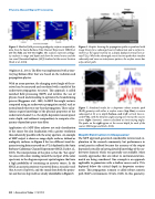
Figure 5. Matched field processing ambiguity surfaces computed for Figure 5. Graphic showing the propagation paths as predicted with
data from the santa Barbara (CA) channel Experiment (SBCX) at image theory for a submerged source (submarine) and a surface in-
233 Hz (left) and 338 Hz (right). The surfaces represent ambigu- terferer as the signal received on a deeply deployed vertical line ar-
ity surfaces in range and depth and show the towed source and the ray (VLA). while the submerged source has two paths that interfere
tow Vessel (Acoustic Explorer [AX]) localized at the correct location coherently and cause an interference pattern, the surface source has
(Zurk et al., 2003). only a direct path.
vru........v-pr Vrlruforlriluulu
(Ogden et al., 2011). The filter was implemented with a time- ' :
varying Kalman filter that was based on the radiation and ° V i 1;,
propagation physics. l ‘ \ §.i E
.. {fl 5
With an array aperture, the changing arrival angle of the re- _Y ,,:L',‘,:,'_,,, 51
ceived can be measured and correlated with a model of the ' . .‘ """' 7»
_ _ _ _ -r.r..r....n 1 ,__ ,, w....,,,,.r
underwater propagation structure. Tlus approach is called I: ' / __ Iewm 4:.-so ml
matched field processing (MFP) and involves the use of E {Q
physics-based understanding to optimize the beamforming a ‘v!
process (Baggeroer et al., 1991). In MFI’, the weight vector is an N u E _ _ M Q _ X’
computed using an underwater propagation model, such as "M """
normal mode theory or ray-based propagation. These calcu- Figure 7. Simulated results fizr a deepwater robust acoustic path
lations require knowledge of the physical properties of the (RAP) Z€'”"9"}’ Will‘ elm?’ “ 5’"f‘‘“ 50“m’5 (MP: “"_2) 07_S014Y€e
underwater Chame1(i_e__the dePth_dePendem sound speed, submerged at so m m depth (bottom, red). Left-yertrcal time re-
. . . cord (VTR), with the elevation angle Varylrigover time as the sources
water depth, and sediment composition) to compute a fre- . _ . . .
_ move. Right. harmonic content calculated at t1me—Vl1r}/mg angles.
quencv-dependent space-“me film The peaks on the right appear at the correct depth for each of the
M C d Z k, 2013 .
Application of a MFI’ filter achieves not only classification Source“ 5 mg“, an In J
of the source but also localization with a greater resolution
than inherently possible with the array aperture. An example Depth Estimation in Daapwatar
of MFI’ output is shown as range-depth surfaces, defined as The MFI’ approach generated considerable interest and ex-
ambiguity surfaces, in Figure 5 for two different tonal £re- ploration in the research community, but performance in
quencies using data measured on a VLA deployed in the Santa actual practice suffered because the accuracy of the output
Barbara (California) Channel Experiment (SBCX; Zurk et. al., depended critically on having detailed knowledge of the un-
2003). The interpretation of the plots is that the “hot spots” derwater channel, which was generally not available. More
(or areas with colors tending toward the red part of the color recently, approaches that are robust to environmental mis-
spectrum) in the diagram represent spatial regions that have match are being considered. One example is an approach
a high probability of containing an acoustic source. hi the applicable to geometries with a shallow source and a VLA
SBCX, an acoustic projector was towed from a research vessel deployed below the critical depth in deepwater environ-
(the Acoustic Explorer), and the sound from both the projec- ments. This propagation scenario is called robust acoustic
tor and the tow ship itself are clearly identifiable in Figure 5. path (RAP) environments (Urick, 1983). In this geometry,
si: 1 AI:uuI:l:I Tbday 1 raiizois