Page 30 - Fall2019

Computational Acoustics in Oceanography
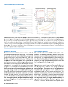
Figure 2. Shallow-water modal dispersion. Top left: an emitted sound waveform such as from a whale (central frequency of 50 Hz). Bottom left: received signals at three ranges (5, 15, and 30 km; r) after propagation in a shallow ocean of 100 m depth (about 3 wavelengths), wherein the sound interacts continually with the seabed and surface, effectively creating a waveguide. Use of a reference wave speed (c0 ) and reduced time (t − r/c0 ) places each signal initiation at zero. The interference of slightly upgoing and downgoing waves makes modes. Each mode is a standing wave in the vertical (top right) and propagates horizontally as a cylindrical wave but with a frequency-dependent group speed (bottom right). The scenario of variable group speed is called dispersion. As seen in the simulated waveforms, dispersion tends to lengthen the signal and to separate modes as range increases.
Simulation Methods
There are numerous simulation methods in use, and each has strengths and weaknesses. Jensen et al. (2011) present the methods, explain the theory behind them, and provide application examples. Often, the weaknesses stem from the short wavelength of underwater sound with respect to ocean depth and width. For example, the 3-D solution for time-harmonic acoustics, available using the finite-element method for a volume with imposed absorbing or radiating boundaries, is unreasonable for the ocean because many grid points per wavelength are required in many scenarios, and the needed matrix solution methods are challenging for areas large enough to make a reasonable study. Facing this challenge, underwater acousticians have developed and/ or refined alternatives. The already mentioned ray method is useful for many purposes. Normal mode and parabolic equation (PE) methods are other primary players for large- scale simulations. Each of the methods is elegantly based on the underlying theory of sound propagation and applied math methods.
Normal Mode Method
This is based on the standard differential equation math method of the separation of variables, where the vertical and horizontal structures of the sound field are given by different functions that are multiplied together to form the full solu- tion. The vertical functions are the normal modes, which are trapped in the ocean waveguide bounded by the surface and the (usually partially absorbing) seabed.
Figure 2 shows mode shapes and how modes disperse, not all propagating with the same group speed. The modes propagate horizontally and can exchange energy (coupled-mode propagation) or not (adiabatic-mode propagation; mode-by-mode energy conservation). The adiabatic approximation gives the correct solution for a flat-bottomed ocean with a uniformly layered seabed, no waves, and a uniformly layered water but gives results with ever-decreasing accuracy as feature complexity is added to approach realistic conditions. The key to applying either technique is ensuring that the errors are acceptably small.
30 | Acoustics Today | Fall 2019