Page 31 - Fall2019

The application of the separation method to waves dates to nineteenth century studies of waves in layered media (e.g., seismic waves) and thence to quantum mechanics, where the modes are the energy states of atoms or mol- ecules. Coupled-mode propagation, with energy exchange as sound moves away from a source, is analogous to time- dependent molecular energy states (think flames, mercury vapor lamps). Confusingly, mode propagation is sometimes treated with ray tracing (e.g. Heaney et al., 1991).
Parabolic Equation Method
This uses a trick to solve the Helmholtz equation. This equa- tion results from imposing a single frequency (sine wave in time) while working with the wave equation. Making the further restriction that sound moves toward or away from point source in cylindrical coordinates, or in one direction along one axis for Cartesian coordinates, yields the parabolic wave equation. This has the troublesome square root operator, which requires another approximation before solving is pos- sible. Various approximate forms of the operator are in use.
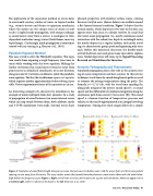
An interesting example of a discovery by simulation is the example of mode multipath from duct emission. In a study of propagation of sound between two ocean internal waves, which can trap sound between them, both adiabatic mode and 3-D PE simulations were made. Internal waves share
physical properties with familiar surface waves, existing because stratified water (denser below) can oscillate around a flat-layered internal condition. Figure 3 shows that the normal modes, which disperse in two ways in the duct, can appear more than once at a distant receiver. In usual shal- low-water ocean propagation (i.e., nearly continuous sound interaction with the seabed, low depth to wavelength ratio), the modes disperse in a regular fashion, each mode travel- ing at a characteristic group speed and appearing only once each. Before this numerical discovery, the double-mode arrivals had been seen and given many speculative explana- tions. Modal dispersion will come up in Signal-Processing Research and Simulations for Inversion.
Acoustic Tomography and Thermometry
Simulated propagation plays a key role in the acoustic sens- ing of ocean temperature and heat content. In this inverse technique, travel times for sound along known paths are used to estimate the average temperatures along the paths. The formula is t = ∫SR (1 ⁄ c)ds, with the travel time equaling the along-path integral of the inverse sound speed (c is sound speed, and the differential [ds] indicates integration along the continuous path from source [S] to receiver [R]). The sound speed is a known function of temperature, pressure and salinity, so this can be approximated as an integral involving temperature. Sensing over short ranges allows for a simple
Figure 3. Simulation of sound field strength between two ocean internal waves in shallow water, with the waves (part of a three-wave packet) tapering to zero away from the source. The wavy surface marks the (smooth) boundary between warm water above and cold water below. Left: field at one frequency as per Figure 1. Right: arrival time series at a few locations for a pulse-style simulation. Mode one appears twice at bottom right, while it is absent in the frame to the left. From Lin et al., 2009.
Fall 2019 | Acoustics Today | 31