Page 22 - Summer2020

FEATURED ARTICLE
Solving Complex Acoustic Problems Using High-Performance Computations
Gregory Bunting, Clark R. Dohrmann, Scott T. Miller, and Timothy F. Walsh
Introduction
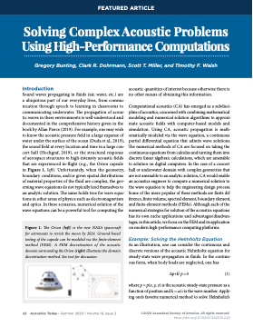
Sound waves propagating in fluids (air, water, etc.) are a ubiquitous part of our everyday lives, from commu- nication through speech to learning in classrooms to communicating underwater. The propagation of acous- tic waves in these environments is well-understood and documented in the comprehensive history given in the book by Allan Pierce (2019). For example, one may wish to know the acoustic pressure field in a large expanse of water under the surface of the ocean (Duda et al., 2019), the sound field at every location and time in a large con- cert hall (Hochgraf, 2019), or the structural response of aerospace structures to high-intensity acoustic fields that are experienced in-flight (e.g., the Orion capsule in Figure 1, left). Unfortunately, when the geometry, boundary conditions, and/or given spatial distributions of material properties of the fluid are complex, the gov- erning wave equations do not typically lend themselves to an analytic solution. The same holds true for wave equa- tions in other areas of physics such as electromagnetism and optics. In these scenarios, numerical solution of the wave equations can be a powerful tool for computing the
acoustic quantities of interest because otherwise there is no other means of obtaining this information.
Computational acoustics (CA) has emerged as a subdisci- pline of acoustics, concerned with combining mathematical modeling and numerical solution algorithms to approxi- mate acoustic fields with computer-based models and simulation. Using CA, acoustic propagation is math- ematically modeled via the wave equation, a continuous partial differential equation that admits wave solutions. The numerical methods of CA are focused on taking the continuous equations from calculus and turning them into discrete linear algebraic calculations, which are amenable to solution on digital computers. In the case of a concert hall or underwater domain with complex geometries that are not amenable to an analytic solution, CA would enable an acoustics engineer to compute a numerical solution to the wave equation to help the engineering design process. Some of the more popular of these methods are finite dif- ference, finite volume, spectral element, boundary element, and finite-element methods (FEMs). Although each of the numerical strategies for solution of the acoustics equations has its own niche applications and advantages/disadvan- tages, in this article, we focus on the FEM and its application on modern high-performance computing platforms.
Example: Solving the Helmholtz Equation
As an illustration, one can consider the continuous and discrete versions of the acoustic Helmholtz equation for steady-state wave propagation in fluids. In the continu- ous form, when body loads are neglected, one has
Δp+k2 p = 0 (1)
where p = p(x, y, z) is the acoustic steady-state pressure as a function of position and k = ω/c is the wave number. Apply- ing one’s favorite numerical method to solve Helmholtz’s
©2020 Acoustical Society of America. All rights reserved.
Figure 1. The Orion (left) is the new NASA spacecraft for astronauts to revisit the moon by 2024. Ground-based testing of the capsule can be modeled via the finite-element method (FEM). A FEM discretization of the acoustic domain surrounding the Orion (right) illustrates the domain discretization method. See text for discussion.
22 Acoustics Today • Summer 2020 | Volume 16, issue 2
https://doi.org/10.1121/AT.2020.16.2.22