Page 24 - Summer2020

HPC FOR ACOUSTICS
density that vary with vertical position in underwater or atmospheric acoustics).
By contrast, finite-difference approaches employ a struc- tured grid that cannot easily capture curved interfaces. Boundary element methods present a dense linear system of equations, which makes coupling with finite-element- based structural models challenging because the latter present a sparse system of equations. In fairness, these alternative methods also have their own advantages over FEMs in certain applications. However, a common theme is the emergence of HPC resources and the benefits that are being presented to any numerical approach for solv- ing acoustic problems.
Finite-Element Method
The FEM has been widely used as a tool for solving the acoustic wave equation. One of the earliest references is from Gladwell (1965), quickly followed by several follow- on efforts (Craggs, 1971). Additional references involving the coupling of an acoustic fluid with a structure fol- lowed in the late 1960s and early 1970s (Zienkiewicz and Newton, 1969; Craggs, 1972). More recent surveys on FEMs for acoustics and structural acoustics provide comprehensive technical reviews on the application of FEMs for solving acoustics problems (Atalla et al., 2017).
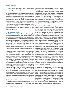
Finite-element technology solves partial differential equa- tions (PDEs) by turning them into linear algebra. The FEM discretizes the physical domain of a problem into a finite number of elements. This discretization process is illustrated in Figure 1, right, for the Orion space cap- sule. In this case, the goal is to understand the structural response of the Orion capsule to high-intensity acoustic excitation as would be experienced in flight. The continu- ous physical domain (box) containing the Orion space capsule in Figure 1, left, is subdivided into a collection of elements in Figure 1, right. The solution is approximated by a polynomial with unknown coefficients, defined locally on each element, and is substituted into a suit- able integral representation of the PDE. The result of this approximation methodology is a linear system of equa- tions to be solved for the polynomial coefficients. Each of these unknowns is referred to as a degree of freedom.
Getting Around Moore’s Law
Gordon Moore (1965) observed that the speed of a com- puter processor doubles about every two years. This
became known as Moore’s law and served as a target for computer chip manufacturers for several decades. During the reign of Moore’s law from 1975 to 2012, larger computational problems could be solved by waiting for a faster processor to be produced. However, Moore’s law could not reign forever because the physical limits of the microelectronics prevented such perpetual growth. Rather than wait for a faster processor, it became neces- sary to use many processors working together to solve larger problems; thus parallel computing is born.
The Advent of Parallel Computing
The early work in parallel computing for acoustics started in the 1990s and consisted of using many CPUs to solve a given problem. In the case of a finite-element solution of the wave equation, the approach was a divide-and- conquer strategy (aka domain decomposition), where the individual finite elements were evenly distributed across the CPUs and the solution of the global set of algebraic equations would be accomplished by many CPUs work- ing in parallel. With the continued demise of Moore’s law, manufacturers are now producing GPU-based com- puting platforms. A single GPU can have thousands of processor cores compared with tens of CPU cores per computational node. Seymour Cray, the father of super- computing, once remarked, “If you were plowing a field, which would you rather use: two strong oxen or 1024 chickens?” (Cray, 2020). This antiquated quote reflects the opinion that it would be more advantageous to have one fast processor rather than restructuring work to be accomplished in a massively parallel fashion. Modern HPC is finding a way to harness the power of the chickens when the oxen are unavailable. Heterogeneous comput- ing environments, where CPUs, GPUs, and possibly other processors coexist on a single piece of hardware are the future of scientific computing.
Key points for the parallelism of work are synchroniza- tion and independence. Tasks to be executed in parallel need to be independent from each other so that it does not matter which one gets completed first. Synchronization points in an algorithm provide a waiting point where all parallel tasks can meet up and exchange any information that might be needed for future work. Current models for heterogeneous computing rely on CPUs to organize and divide tasks to be parallel processed on the GPU. Hard- ware configurations dictate that multiple CPUs must be able to execute tasks simultaneously on a single GPU.
24 Acoustics Today • Summer 2020