Page 28 - Summer2020

HPC FOR ACOUSTICS
Aeronautics and Space Administration, 2019) in the middle of the vibroacoustic test facility (VATF) of Sandia National Labs (Schultz et al., 2015). We note that this is purely a numerical study, not an actual experimental test. The VATF is a rectangular box 6.58 m × 7.50 m × 9.17 m, making the volume ratio of capsule to room approximately 0.1. Acoustic excitation to the 140 dB level is provided by a 0.1-m2 loudspeaker in the bottom corner of the room. It provides a sinusoidal acoustic velocity loading with an amplitude of 3.4 m/s and a frequency of 350 Hz.
The accuracy of a finite-element solution is dependent on the size of the elements used to obtain the solution. In acoustics, the element size used in the mesh will limit the frequencies resolved. For instance, computing a sound field using finite elements would require the mesh size
h= (3)
where h is the size of the finite element, c0 is the speed of sound in air, fmax is the highest frequency requested, and λ is the number of elements per wavelength needed. Typi- cally, for low-frequency excitation, we select λ = 10 for linear hexahedral elements. Fewer elements can be used
in conjunction with high-order polynomial interpola- tion as the basis functions that are able to approximate a waveform with less error, but for simplicity, we do not cover those details here.
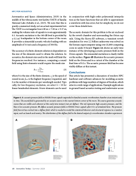
The acoustic domain for this problem is the air enclosed by the reverb chamber and surrounding the Orion cap- sule. Using the Sierra-SD software, a transient reverb simulation for over 2.2 billion unknowns was solved on the Serrano supercomputer using over 22,000 computing cores in under 8 hours! Figure 4A shows an early time instance of the developing acoustic pressure field on the Orion capsule. The sinusoidal excitation is clearly visible on the surface. Figure 4B illustrates the acoustic pressure field on the Orion and in a cutout of the chamber at the final time of 0.2 s. The acoustic pressure field has become visibly diffuse at this instant.
Conclusions
This article has presented a discussion of modern HPC hardware and software advances for modeling acoustic problems with large numbers of degrees of freedom, which arise in a wide range of applications. Example applications in ground-based acoustics testing and underwater acous-
Figure 4. A: acoustic pressure field on NASA’s Orion capsule suspended in Sandia’s acoustic reverberation chamber at an instant early in time. The sound field is generated by an acoustic source in the nearest bottom corner of the room. The source generates acoustic waves that are visible and coherent at this early time instant (not yet diffuse). The red represents high acoustic pressure, and the blue is low acoustic pressure. B: diffuse acoustic pressure field on NASA’s Orion capsule after 0.2 s of simulated time. The pressure field from A has evolved into a diffuse field, which is needed to model the statistical behavior and structural response to a random input, such as launch and reentry. The distribution of this diffuse field is the desired output of a reverberation chamber experiment.
28 Acoustics Today • Summer 2020