Page 56 - Fall2021

DAVID M. GREEN
Chuck generated a temporal sequence of 10 brief (e.g., 40-ms), equal-amplitude tones presented sequentially, each with a different randomly determined frequency spaced far enough apart to be distinguishable. In one set of experiments, two 10-tone patterns were presented in succession, with the two patterns being the same or one pattern having the frequency of just one of the tones changed. The listeners determined whether the two pat- terns were the “same” or “different.”
If highly trained listeners were presented the same 10-tone pattern (same frequency components fixed over time) over and over, they could, after considerable prac- tice, distinguish a frequency difference for each tone in a pattern nearly as well as they could when the tones
were presented alone rather than as part of a pattern. However, when the frequencies of the 10 tones were not fixed over time but varied randomly, the listeners were uncertain about the spectral changes that occurred. The more aspects of the patterns that were randomly varied, the greater the uncertainty and Watson (2005) showed that discrimination performance for 10-tone patterns depended on the amount of uncertainty. It did not take Murray long to get Dave interested in the role uncertainty played in these 10-tone pattern experiments.
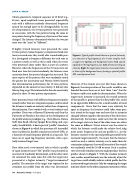
Dave presented tones with different frequencies simulta- neously rather than in a temporal sequence, and he asked the listeners to make an intensity rather than a frequency discrimination. Dave worked with several students and postdocs (Dave was at Harvard University and then the University of Florida at this time) in the development of the profile analysis paradigm (e.g., Chris Mason, Donna Neff, Tom Buell, Murray Spiegel, Bruce Berg, and, espe- cially, Gerald Kidd). A basic spectral “profile” stimulus is shown in Figure 6 in which the spectrum of 5 sinusoidal tones is plotted as decibel sound pressure level (SPL) as a function of tonal frequency plotted on a log scale. The tones are at equal log-frequency intervals, with a spec- trally centered target tone.
Dave often used a two-interval task in which a profile of equal intensity tones (“flat” profile) was presented in one interval (randomly determined), and the other inter- val contained the same tones but with the target tone presented at a higher intensity (“target-incremented” profile). The intensity of the target tone required to dis- criminate one profile from the other was determined.
However, if the stimuli were just like those shown in Figure 6, the interpretation of the results would be con- founded because there are at least three “cues” that the listeners could use to make the discrimination. When the target tone’s intensity is increased, the overall intensity of that profile is greater than the flat profile (this could be an appreciable difference for a small number of tonal components). Given that the tones were relatively far apart in frequency, the listeners could (after some prac- tice) attend to the target tone and note that its intensity changed without regard to the intensity of the other tones. Alternatively, the listeners could note that the intensity of the target relative to that of the other tones was either the same or different. Dave’s interest was the extent to which the listeners could make the relative level judg- ment across frequency for any one profile (i.e., are the listeners sensitive to the spectral profile generated by the increased target intensity?). To ensure that the listeners could use only a relative intensity cue to make their dis- crimination judgment, the overall intensity of the sounds was randomly roved by 20 dB or more. Such a random rove of overall stimulus intensity might produce the four profiles shown in Figure 7. With the random intensity rove, neither overall intensity nor the intensity of just the target tone could reliably indicate which profile had the incremented target intensity. Only by comparing the target intensity relative to the other component intensities within
Figure 6. Typical profile stimuli shown as spectra (intensity as a function of log frequency) of a 5-tone complex with a target tone (green) and background tones (red) spaced regularly on the log-frequency axis. Left: all tones are of equal intensity. Right: the target tone’s intensity is increased relative to those of the background tones, forming a spectral profile. SPL, sound pressure level.
56 Acoustics Today • Fall 2021