Page 48 - Winter 2020

ONE SINGER, TWO VOICES
very wide limits. We can vary the shape of the tongue body, the position of the tongue tip, the jaw and lip open- ings, the larynx height, and the position and status of the gateway to the nose, the velum.
Let us now more closely examine the shape of AMH’s VT as documented in the MRI video. It is evident from Figure 6 that AMH produced overtone singing with a lifted tongue tip, so the tongue tip divided the VT into a front cavity and a back cavity. Our first target is the back
cavity posterior to the raised tongue tip.
The formant frequencies associated with a given VT shape can be estimated from the VT contour. Several investigations have examined the relationship between the sagittal distance separating the VT contours and the associated cross-sectional area at the various positions along the VT length axis (see, e.g., Ericsdotter, 2005). Hence it was possible to describe the shape of the back cavity for each FE in terms of an area function that lists the cross-sectional area as a function of the distance to the vocal folds.
The next question concerns the front cavity, anterior to the raised tongue tip. The cavity between palatal constric- tion and the lip opening looks like, and can be regarded as, a Helmholtz resonator, a cavity in front of the tongue
tip and a neck formed by the rather narrow lip opening (Sundberg and Lindblom, 1990; Granqvist et al., 2003).
The area of the lip opening was measured in a front video recorded when AMH produced the same overtone series as for the MRI video. The length of the lip opening was docu- mented in the MRI video. These measures plus the frequency of the third formant used for the inverse filtering analysis allowed us to use the Helmholtz equation for calculating the front cavity volume. The validity of this approximation was corroborated in terms of a strong correlation between the measured length and the volume of the front cavity.
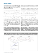
The formant frequencies of the entire VT could be calcu- lated by a custom-made software, Wormfrek (Liljencrants and Fant, 1975). Figure 8 shows the transfer functions with the formant frequencies for three FE values: 1,096, 2,166, and 3,202 Hz. In Figure 8, the arrows highlight the close proximity of F2 and F3. In Figure 8, bottom, F1, F2, and F3 are plotted as a function of FE. The trend lines show that F2 and F3 have similar slopes and intercepts differing by about 220 Hz.
We note that the F1, F2, and F3 predictions parallel the formant measurements made using inverse filtering (Figure 7). Here, a somewhat wider distance separates F2 from F3 than what was shown in Figure 7. The common
Figure 8. Top: Wormfrek software displays of the transfer functions for the lowest, a middle, and the highest FE (left, center, and right, respectively). Bottom: associated values of F1, F2, and F3 as a function of FE. Lines and equations refer to trend line approximations.
48 Acoustics Today • Spring 2021