Page 41 - Winter2021

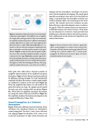
ranging) and the atmospheric counterpart of oceanic sonar (sound navigation and ranging). The sound signal, typically consisting of a short pulse in the low kilohertz range, is transmitted into the atmosphere and then scat- tered by turbulent eddies, thus returning an echo to the receiver. The transmit and receive antennas use para- bolic reflectors or phased loudspeaker arrays to enhance the signals. When the transmit and receive antennas are at different locations, the system is bistatic; when anten- nas are colocated, it is monostatic. Sodars provide wind profiling up to altitudes of about 2 km above ground as well as information on the intensity of temperature and velocity fluctuations.
Figure 4. Amplitude and phase fluctuations for scattered signals as depicted on polar diagrams. Three different cases, arranged by the strength of the scattering, are shown. These cases involve data for amplitude and phase fluctuations in different meteorological conditions (Kamrath et al., 2021). a: For weak amplitude and phase fluctuations, samples (blue and orange dots) are in a small arc on the unit circle and correspond to samples before and after an atmospheric event that caused a transition in the signal behavior. Samples correspond to those from the signal’s complex time series, whose normalized amplitude and phase correspond to distance from the origin (black dots) and polar angle. b: For still small amplitude fluctuations and large phase fluctuations, samples spread around the unit circle, creating a bull’s-eye pattern. Dots appear as “clouds” due to the high point density. c: For strong amplitude and phase fluctuations, center of the unit circle fills in.
Figure 5. Practical situations where turbulence significantly affects sound propagation. a: Acoustic remote sensing of the atmosphere with sonic detection and ranging (sodar). b: Sound scattering into a refractive shadow zone. c: Acoustic pulse propagation. d: Coherence loss of acoustic signals. See text for detailed description of each situation.
Polar grids (also called phasor diagrams) provide an insightful characterization of the amplitude and phase fluctuations. Figure 4 shows distinctive patterns produced for differing scattering strengths. For weak (unsaturated) amplitude and phase fluctuations, complex signal samples are confined to a small arc on the unit circle (Figure 4a). When the amplitude fluctuations are still small but the phase fluctuations are large, the samples spread around the entire unit circle, creating a bull’s-eye pattern (Figure 4b). When both the amplitude and phase fluctuations are strong, the center of the unit circle fills in (Figure 4c). The amplitude and phase fluctuations also depend on the strength of diffraction (Colosi, 2016).
Sound Propagation in a Turbulent Atmosphere
Figure 5 illustrates different practical situations where
turbulence has significant impacts on atmospheric sound propagation. The first is sodar (sonic detection and ranging; Figure 5a) (Bradley, 2010). Sodar is the acoustical counterpart of radar (radio detection and
Winter 2021 • Acoustics Today 41