Page 37 - Summer2022

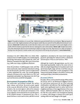
Figure 3. Examples of interference in acoustic data. All plots show grayscale decibel levels of received power. Top: spectrogram of passive acoustic data. Significant features of the spectrogram include ship noise (point B) and broadband electrical power noise (point A). Bottom left: broadband echo sounder data that include acoustic modem noise (point C) and acoustic Doppler current profiler (ADCP) interference (point D) that obscures scattering from water column features. Bottom right: beamformed acoustic array data indicating the direction of arrival (bearing) in degrees of energy versus time. Ship transects are visible and change in bearing versus time (point B). Acoustic modem noise is also present in the bearing color plot (point C, vertical dashed lines). (Gassman et al., 2017; Miksis-Olds et al., 2018). Other common sources of anthropogenic noise include airguns, pile driving, wind turbine noise (Amaral et al., 2020), and vibrations transmitted through other types of structures (e.g., traffic near a dock, oil platform vibrations). Given the prevalence of anthropogenic noise, and ship noise in particular, many researchers have been working over the last decade to use these “sources of opportunity” to better understand the ocean. This includes gleaning estimates of biomass in the ocean (Haris et al., 2021) and temperature and salinity (e.g., Kuperman et al., 2017) via a process known as acoustical tomography. Environment Propagation Effects The underwater environment includes the surface, water column, and bottom. Received acoustic signals in the ocean are affected by all three. In all underwater acoustics, the received signal is affected by transmis- sion loss, which is the spread and attenuation of the source signal by environmental factors and absorption. In the simplest estimate of transmission loss, a line is drawn between a source and receiver, and the received amplitude is calculated as the source level minus the geometric spreading loss (spherical and/or cylindrical) and absorption (Francois and Garrison, 1982). Although this would be the approximate case for a uni- form sound speed profile, sound in the ocean curves, is reflected, and gets trapped based on boundaries and sound speed versus depth, range, and time. In all these cases, an essential fact of underwater acoustic propagation is that temporal and spatial changes in the surface, bottom, and sound speed impact instrument measurements. Boundary Effects Boundary effects, such as sound bouncing off the surface, the bottom, and ice, are illustrated in Figure 4. Surface, ice, and bottom interactions all can cause scattering, reverberation, and reflection. The resulting signal mul- tipath varies significantly based on surface and bottom roughness and slope or from jagged features of the ocean bottom. Additional boundary effects are driven by the fact that the ocean seabed is not homogenous; layering is common, with changes in density and sound speed causing reflections and changes in the signal. Summer 2022 • Acoustics Today 37