Page 16 - Fall 2005

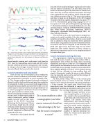
Fig. 4. Travel times measured on the 1–5 Mm-long acoustic paths (red and blue) compared to travel times predicted using the JPL-ECCO ocean model (green). See Fig. 2 for path identification. Six to twelve rays are resolved and identified on each acoustic path. (From Ref. 8 © 2004 Institute of Electrical and Electronics Engineers.)
showed modest warming and a weak annual cycle from late 1997, when the transmissions started, until early 2003, when the path cooled abruptly and a strong annual cycle returned. In retrospect, these changes stemmed from the warming of the central Pacific that occurred in this interval.
Acoustic thermometry and ocean models
From the very start we envisioned a close coordination between acoustic thermometry and satellite altimetry to pro- vide complementary constraints on ocean circulation mod- els. This strategy combines the good horizontal resolution of altimetry and the depth resolution and good time resolution of tomography. In order to use acoustic path integral data as constraints on ocean models, one must first be able to use the model output to construct realistic sound-speed fields for use in acoustic propagation calculations (the forward problem). Until quite recently the vertical resolu-
tion of ocean general circulation models was too coarse to allow construction of realistic sound-speed profiles. Modern models, however, such as that imple- mented by the ECCO Consortium (Estimating the Circulation and Climate of the Ocean), finally have the vertical resolution needed for acoustic propaga- tion calculations, allowing for straight- forward comparison of measured and predicted travel times.
Nonetheless, sound speeds derived
from the ECCO model initially gave unphysical results when used for acoustic calculations. The time mean state of the model was therefore replaced by fields from the World Ocean Atlas. Once this was done, measured travel times and travel times computed from the model are similar, although signif- icant differences remain (Fig. 4).8 The ocean state estimate used here is based on an integration of the MIT General Circulation Model in a global configuration that spans 75o S to 75o N, with latitudinal grid spacing ranging from 1/3o at the equator to 1o at the poles and longitudinal grid spacing of 1o. The model assimilates a variety of satellite and in situ data and data products, including TOPEX/POSEIDON altimetric data, World Ocean Circulation Experiment (WOCE) hydrography, eXpendable BathyThermograph (XBT) sec- tions, and Argo float data.
The next step is to use the travel times as integral con- straints on the model variability. If the data estimated by the model do not match the observations, then the ocean model state is adjusted to bring the model into better agreement with the data. Using modern ocean state estimation methods, the acoustic data can be compared to and ultimately com- bined with upper-ocean data from Argo and sea-surface height data from satellite altimeters to detect changes in abyssal ocean temperature and to test the complementarity of the various data types.
Acoustic thermometry and Argo float data
The Argo program is deploying autonomous floats that drift with the ocean currents at a depth of about 2000 m. Approximately every 10 days the floats surface, measuring temperature and salinity as they rise. The temperature and salinity profiles are transmitted to shore via satellite link, and the float then returns to depth. The goal is to have about 3000 floats deployed globally at all times, with a nominal spacing of about 300 km. Although the Argo profiling floats and acoustic thermometry sample the ocean in quite different ways, the Argo data can be used to construct line averages for comparison with the acoustic data.
All float profiles within 300 km of the acoustic path from the Kauai source to receiver k were first extracted. Figures 5 and 6 show the horizontal and vertical sampling in a 10-day snapshot. The annual mean World Ocean Atlas temperatures were then subtracted to remove most of the geographical variations in temperature and to focus on the “anomalies.” The resulting temperature profile anomalies
were depth-averaged, and these in turn were averaged together on 10-day inter- vals—insofar as this was possible (many of the floats early in the time series are shallow). The acoustic travel time measurements were inverted using a simple statistical ocean model consist- ing of six vertical modes, including a mixed layer, to represent vertical vari- ability and a red spectrum with 20 wave numbers to represent horizontal vari- ability; the variance in the main ther- mocline was ~ 1oC.
“It is inconceivable to us that oceanographers (and other marine mammals) should not take advantage of the fact that the ocean is transparent to sound.”
14 Acoustics Today, October 2005