Page 28 - January 2007

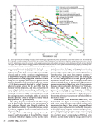
Fig. 2. Curves representing the nominal high (solid gray) and low (dashed gray) magnitude of the pressure spectral density of underwater ambient noise. The nominal high curve is based on a combination of heavy shipping activity plus sea state 6, and the nominal low curve is based on a combination of light shipping activity plus sea state 0 (see text for explanation on construction of curves). Several examples of measurements of the ambient noise pressure spectral density are plotted with references identified in the legend. (These represent different averaging periods and measurement bandwidths, and use of either symbols or lines does not reflect frequency resolution of meas- urements.) The spectral density of thermal noise is shown in the lower right corner for reference.
underwater ambient noise in the 10–100,000-Hz band.
The starting frequency of 10 Hz is motivated more by simplicity and need to limit the scope of this discussion. The infrasonic band of < 10 Hz is also more strongly influenced by shallow water waveguide effects that establish a cutoff fre-
1
quency for effective sound propagation. However, it is worth
noting here that in pelagic, open waters, the general trend for frequency dependence and spectral level within the nominal 1–10-Hz band is reasonably described by the Holu Spectrum (observed to apply between 0.4 Hz and 6 Hz), from the Hawaiian word for deep ocean,13 and which is shown for ref- erence in Fig. 2. Ambient noise in this spectral band is asso- ciated with the dynamics of ocean surface waves. Shorter wavelength ocean waves exhibit a saturation beyond which they no longer increase in waveheight, and this is mirrored in the Holu Spectrum insofar as the spectral density remains roughly constant for a given frequency.
The ending frequency of 100,000 Hz (100 kHz) is large- ly set by thermal noise generated by the random motion of water molecules. Thermal noise ultimately establishes the lower limit of measurability of pressure fluctuations associat- ed with truly propagating sound waves, and is also shown for reference in Fig. 2.
In regions of the world with high shipping densities, the frequency band between about 10 Hz and 200 Hz is primari- ly associated with distant shipping activity, and this source
typically constitutes the largest anthropogenic contribution to underwater ambient sound in terms of mean-squared
1,6
6
frequency, which is reflected in the Wenz curves. Wind-gen-
erated noise largely results from bubbles created in the process of wave breaking. At lower frequencies (< 500 Hz) it is the oscillation of bubble clouds themselves that are consid- ered to be the source of sound,16,17 while at higher frequencies the excitation of resonant oscillations by individual bubbles is
18,19
illustrate both some degree of consistency, and discrepancy, with the two curves describing nominal high and low noise pressure spectral density. These data sets represent different averaging periods and measurement bandwidths (discussion on the related topic of frequency resolution and spectral vari- ance, which can be found in many standard texts, is beyond the scope of this article). The data curve for a wind speed of 2–4 m/s (4–8 knots),20 corresponding to WMO sea state between 1 and 2, is clearly parallel to our high and low curves
The majority of the noise power radiated into the
pressure.
water by surface ships comes from propeller cavitation. Above 200 Hz, depending on wind speed, and extending up to ~100 kHz, wind-generated sea surface agitation governs much of the ambient noise field. Wind-speed related noise rather consistently shows an approximate 5 dB reduction in average pressure spectral density per factor of two increase in
the source of sound.
Several ambient sound data sets are shown in Fig. 2 to
14,15
26 Acoustics Today, January 2007