Page 16 - April 2008

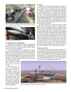
Fig. 7. Close up of infrasound sensor connected to four porous hoses. The porous hoses act as a windscreen for the sensor and are connected to a central manifold (the white segment) at the top of the sensor.
Fig. 8. Orion rocket attached to launch rail.
The distribution of recorded signals
Signals from the explosions of the three experiments were recorded at array stations to a range of approximately 900 km. Twenty four of the thirty stations recorded signals from at least one of the explosions.
The spatial distribution of the observations, as seen in Figs. 3 to 5, provides insight into the dominant propagation mode of the sound. For the September 2005 test (Fig. 3), the predicted zonal wind direction was to the west. Therefore, the station distribution favored this direction, where most of the acoustic energy would be expected to return back to the ground. The observations (green dots) confirm this ducting of acoustic energy—long
range observations (greater
than 400 km) were only
observed in the westward
direction.
The March 2006 test (Fig. 4) is a good example of observations driven by stratospheric winds to the east. In the July 2006 test (Fig. 5), the winds transitioned back to the west and the resulting observations fell in that direction. Further study of these acoustic “footprints” will provide an opportunity to refine understanding of the atmosphere and its effect on acoustic propagation.
Waveforms
Figures 10 and 11 show examples of signals recorded at the two closest arrays, NW70 and VANDAL (less than 100 km), as well as at two arrays further away, GILA and CHIR (100–300 km). The time series in these figures are aligned to the approximate signal onset. The simple pulse-like signals (N-waves) recorded at the two stations at close range (Fig. 10) contrast with the increasing complexity and reduced sig- nal-to-noise ratio (SNR) of the multi-pathed waveforms at the more distant stations (Fig. 11). The two CHIR waveforms for the WSMR3 explosions were separated by only four hours in time, yet the waveforms are quite different—a dramatic illustration of the effects of atmospheric variability on long- range infrasound propagation.
At many stations there were several distinct signal arrivals from each explosion. Signals associated with the explosions were identified based on the expected arrival time, as well as on the stability of azimuth and phase velocity estimates and the value of the F-statistic during the time win- dows of stable azimuth and phase velocity. The beginning and end of such stable data windows were picked manually. Arrival times for stations at close distances (less than 100 km) were also measured manually. Signal parameters were calcu- lated for each apparent discrete arrival in the selected data windows. In addition, root-mean-square (RMS) noise values were measured, both for time windows prior to the first sig- nal arrival as well as in a time window spanning the expect- ed arrival time (for those cases where no signal was observed). Average and RMS wind speed was also calculated from the time windows of received or expected arrivals.
Signal group velocity
The observed group velocity of all signals, defined as the (distance)/(arrival time–explosion time), is plotted in Fig. 12 (where the distance has been corrected for the altitude of the source). For the WSMR2 experiment the signals propagating eastward (with the wind) show increased velocities, whereas in WSMR3 it is just the opposite. These observations are con- sistent with the distribution of observations noted in Figs. 3- 5, as well as with the modeling presented in Fig. 2.
Fig. 9. Rocket trajectories and explosion locations (colored circles) for the WSMR infrasound experiments (view looking to east). White circles indicate the sites of some of the closer recording stations.
14 Acoustics Today, April 2008