Page 9 - Winter 2008

circular rings begin to form that propagate progressively toward the source location. At the focal time, a strong veloc- ity maximum occurs at the source location corresponding to the original input pulse. After the focus, the incoming waves pass through each other, propagating outward until the field becomes diffuse once again [Note that the source transducer is actually located on the opposite side of the plate so as not to interfere with the laser].
The rectangular plate example illustrates the power of the TR process. Instead of multiple reflections/scattering destroying the source reconstruction, they enhance it. Reflectors/scatterers act as image (virtual) sources of a TRM. We show conceptually how this works in the illustrations in Fig. 3. Figure 3a shows a closed cavity that contains a source S, and a single receiver, R. When the source emits a pulse, the pulse travels the paths denoted by the blue colored arrows shown in Fig. 3a [An infinite number of paths actually exist from S to R , but we limit our consideration to one reflection from each wall for illustration purposes]. The first arrival at R will be from the direct propagation followed by the reflec- tion from the top wall and so on, until the reflection from the back wall (on the left) arrives (see Fig. 3b). These five arrivals at R (arriving at five different times) can now be time reversed (see Fig. 3c) and emitted re-tracing their forward paths, as shown by the red arrows in Fig. 3d. The later arrivals of energy are emitted first from R, and the last emission from R corresponds to the direct propagation from the forward step. The four emissions of energy, which reflect from the walls, now arrive at S at the same time that the direct propa- gation arrives (purple colored arrows). Now suppose we remove the boundaries from this experiment and redo the TR broadcast step. To have the focusing that we had inside the cavity, we need sources located at the positions indicated by I1􏰀4 in Fig. 3d. The sources at positions I1􏰀4 are called image (virtual) sources and their positions are determined by
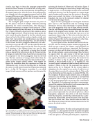
Fig. 4. Photograph of a rectangular aluminum plate used in a Time Reversal study. The overlaid peaks on the plate display the velocity magnitude from actual meas- urements. The overlay-image was taken at the time of focus and the large-ampli- tude red-colored peak corresponds to the original source location.
mirroring the location of R about each wall surface. Figure 3 illustrates the advantage of a closed cavity; despite only using a single receiver—it is as if multiple receivers were used. Each unique path between S and R corresponds to a unique image source location and the more time the receiver is allowed to detect wave arrivals, the better is the focusing in the TR broadcast step due to the increased number of coherent arrivals from the image sources.
Figure 4 shows a photograph of a rectangular aluminum plate used in a TR experiment with the resulting image obtained at the focal time (specifically, the spatial distribu- tion of the magnitude of the out-of-plane velocity) overlaid. Note the well-defined peak in the overlaid image that corre- sponds to the original source location. Note also that other energy exists elsewhere at the focal time (just as is in the experiment shown in Fig. 2). This is due to the fact that the experimental TR focusing process is never perfect due to a variety of factors that lead to energy leakage to other loca- tions. We will discuss later why this may happen.
Up to this point, we have described what we will call stan- dard TR. We now introduce another method of applying TR,
2,9
Figures 5 and 6 illustrate the two methods, in time and space, respectively. For illustration purposes, we show only the direct arrival and a single reflec- tion. In both methods, a source emits energy (Figs. 5a [time], 6a [space]) [Note the color scheme of the first and second arrivals in Fig. 5 corresponds to that shown in Fig. 6.]. The time signal is detected by a receiver (Fig. 5b) located at the position R shown in Fig. 6a. The detected signal is then reversed in time as shown in Fig. 5c. In standard TR, this (reversed) signal is rebroadcast from location R and focuses at location S, shown in Fig. 6b. The associated time signal is shown in Fig. 5d. In reciprocal TR, the reversed signal is rebroadcast from the original source position S and focuses at the original detector position R, as shown in Fig. 6c. This results in the identical focused time signal as in standard TR (Fig. 5d). The reciprocal TR process makes intuitive sense, as the paths traversed in the forward step are retraced in the backward propagation. This is simply a statement of spatial reciprocity, i.e., that the propagation from S to R is the same as that from R to S. Reciprocity is a fundamental principle to wave propaga- tion and the equations that describe it, and a cornerstone in the
which we term reciprocal TR.
TR process (see Limitations section below).
In Fig. 5d, one can see other energy exists that is sym-
metric about the focal time. Since each emitted pulse propa- gates outward spherically, the red colored pulse has a direct propagation component that arrives at the focal location before the focal time, and the blue colored pulse has a com- ponent that reflects from the wall to arrive at the focal loca- tion after the focal time. These arrivals before and after the time of focus are termed side lobes9 and are inherent in the TR process for closed cavities.
Limitations
As mentioned above, TR relies on the principle of spatial reciprocity,10 i.e., the ray paths traversed by a pulse from point A to point B (including reflected paths) will also be traversed if the same pulse is sent from point B to point A. Spatial rec-
Time Reversal 7