Page 25 - Jan2013

must provide
• the transducer size,
• the array geometry,
• the frequency radiated by the pistons,
• a target position somewhere in space in front of the
array, and,
• the sampling volume over which the response is to be
computed.
In our computation, the sampling volume is always a 2D slice aligned with any two of the coordinate axes.
The simulation code was written in the Python language. It makes extensive use of the impressive numerical extension, Numpy, and the large collection of numerical utilities in Scipy. In particular, Numpy made it straightforward to vectorize the innermost computational loop at a substantial time savings. In the code’s final form it took about five minutes to compute the response patterns shown below, each of which represents a 100 by 100 grid of values. This code along with all other elements of the system’s design is available on our wiki:
http://mesoscopic.mines.edu/mediawiki/index.php/Acoustic _Phased_Array
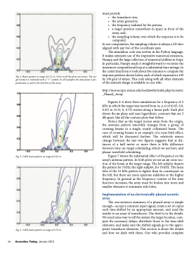
Figures 4–6 show three simulations for a frequency of 5 kHz in which the target was moved from (x, y, z) of (0.05, 0.0, 0.25) to (0.15, 0, 0.75) meters along a linear path. Each plot shows the xz plane and uses logarithmic contours that are 3 dB apart, like all the contour plots that follow.
Notice that as the target moves away from the origin, the antenna pattern smoothly changes from a group of crossing beams to a single, nearly collimated beam. The case of crossing beams is an example of a near-field effect, which will be discussed further. The relatively minor change between the last two figures suggests that at dis- tances of a half meter or more there is little difference between time-on-target scheduling, which we use here, and planar wavefield scheduling.
Figure 7 shows the substantial effect of frequency on the array’s antenna pattern. In both plots we see an xy cross-sec- tion of the beam at the target range. The left subplot depicts the pattern for 5 kHz; the right subplot, for 10 kHz. The main lobe of the 10 kHz pattern is tighter than its counterpart on the left, but there are more spurious sidelobes at the higher frequency. In general as the frequency content of the time function increases, the array must be broken into more and smaller elements to minimize side lobes,
Implementation of an electronically-phased acoustic array
The one-sentence summary of a phased-array is simple enough—accept a common input signal, create a set of copies each time-shifted by an appropriate amount, and send the results to an array of transducers. The devil is in the details. We need some way to tell the system the target location, com- pute the necessary delays, distribute those to the time-shift elements, and make sure the shifted signals go to the appro- priate transducer elements. This section is about the details and how we dealt with them. Our wiki provides complete
Fig. 4. Beam pattern at range of 0.12 m. Units in all the plots are meters. The tar- get location is indicated with a “+” symbol. In all examples the data plane is per- pendicular to and in the mid-line of the array.
Fig. 5. 5 kHz beam pattern at range of 0.25 m.
Fig. 6. 5 kHz beam pattern at range of 0.75 m.
24 Acoustics Today, January 2013