Page 28 - Jan2013

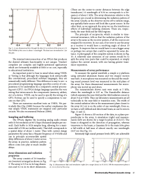
Fig. 11. A one-dimensional slice through the data 0.2 m in front of the array at y=0. The FWHM of this curve is about 1 wavelength. The data were normalized to 1 for this plot.
The internal interconnection of an FPGA that produces the desired ultimate functionality is not unique. Vendors’ compilers are complex and highly-optimized applications which are fortunately available at little or no cost, especially to educational institutions.
An important point to bear in mind when using VHDL or Verilog is that although the languages look syntactically like conventional, procedural software languages, they are semantically vastly different. This difference is easy to see—a procedural programming language specifies a series of com- putations to be undertaken by a computer’s central process- ing unit (CPU). An FPGA design language specifies the very wiring that interconnects the components (memory, adders, etc) of a device. VHDL can be used to specify the wiring of a CPU; Fortran can be used to specify a computation to exe- cute on that CPU.
There are numerous excellent texts on VHDL. We par- ticularly like Chu (2008) because the author emphasises the way simple VHDL statements are mapped onto particular circuits. We also recommend Pedroni (2004).
Sampling and buffering
The FPGAs digitize the incoming analog audio stream with 12-bit resolution at 347.2 ksps (thousand samples per sec- ond). Each buffer is 1024 samples long, allowing for a maxi- mum shift of 2.96 ms (milliseconds). That shift corresponds to a spatial delay of about 1 meter. Thus with current design parameters the array has a Nyquist frequency of 174 kHz and can in principle accommodate spatial
delay differences of about 1 meter across
the array; in practice, radiation pattern
effects come into play at much smaller
delays.
Array dimensions and radiation properties
The array consists of 24 transduc- ers (tweeters) arranged as shown in Fig. 3. The array is 0.3 m in its long dimen- sion and 0.2 m in its short dimension.
(These are the center-to-center distances between the edge transducers.) A wavelength of 0.34 m corresponds to a fre- quency of about 1 kHz. The array dimensions relative to the frequency are crucial in determining the radiation pattern of the array. Clearly, as the observer moves off to infinite range, any spatially finite source will look like a point source. In the other limit, as we approach the array we see the interference effects of individual radiating elements. These are, respec- tively, the near-field and far-field regions.
The principle of reciprocity, which is similar to time- reversal invariance, tells us that the radiation pattern of the array is the same as the receiver pattern, if all the sources are swapped for receivers. In our case, if we were to use the array as a receiver it would have a resolving angle of about 10 degrees. To improve this we would have to use a bigger array or perhaps two arrays that could be separated by some dis- tance. A photograph of the complete system is shown in Fig. 10. A relatively easy extension of our system would be to split the array into parts that could be separated, or simply replace the current mount, with one having greater trans- ducer separation.
Measurements of array performance
To measure the spatial wavefield, a simple x-y platform using extruded aluminum beams and two stepper motors was built. A microphone was mounted on this and the result- ing sound pressure level was measured in the mid-plane of the array. For three-dimensional measurements the micro- phone was moved up and down.
The measurements shown next were made at 5 kHz, where the wavelength is 0.07 m. The Fraunhoffer distance (which separates the near-field and far-field radiation zones) is about 3 m at 5 kHz. Thus our laboratory measurements are all technically in the near-field or transition zone. The width of the central radiation lobe in the measurement plane closest to the array (0.2 m) is on the order of one wavelength. Even so, we have a well-defined and directional beam; as can be seen in Figs. 11 and 12.
Figure 12 shows a 2D section of the data, in a plane per- pendicular to the array. A simulation (right) and measure- ments (left) are shown for a target location at (0.3,0.5). The beam is elongated in the direction of propagation, whereas transverse to the beam, a Gaussian fit to the main lobe gives a full-width at half-max of almost exactly one wavelength (0.07 m) (See Fig. 11).
Extremely high sound pressure levels (SPL) are achievable
Fig. 12. Measurement (left) and simulation (right) for a target (focus) at (0.3,0.5). NB the measurement plane is at .2 m in front of the array.
Electronically-Phased Acoustic Array 27