Page 33 - \Winter 2015

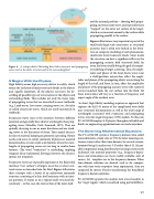
Figure 4. A concept sketch illustrating how both evanescent and propagating waves exist in the elastic structure and in the surrounding fluid.
and the internal partition – showing both propa- gating and evanescent waves and especially those “trapped” on the outer wet surface of the target, which are evanescent normal to the surface while propagating parallel to the surface.
Figure 4 illustrates a very important aspect of the small-scale/large-scale interaction in structural acoustics that is often over-looked in the litera- ture on computer modeling of such phenomena: small-scale local evanescent elastic waves inside the structure can have a significant effect on the propagating acoustic field (scattered field) far away, the latter usually being the goal of comput- er modeling of target scattering. Thus, the ampli- tudes and phases of the local elastic waves near a shell/partition intersection affect the ampli-
It Begins With the Physics
High fidelity means high accuracy relative to reality, which means the inclusion of many structural details in the objects and, equally important, all the physics necessary for de- scribing all possible types of wave motion in the objects and surrounding fluids. This includes not only the many types of propagating waves that are described in most textbooks (e.g., Lamb waves, Love waves, creeping waves, etc.) but also so-called evanescent waves, which are rarely mentioned in textbooks.
Evanescent waves exist at the interfaces between different materials and generally have shorter wavelengths than prop- agating waves (Mindlin, 1960; Zemanek, 1972). They are spatially decaying in one or more directions and are stand- ing waves in the directions of decay. Their spatial decay is not due to material damping or geometric spreading. Nature needs such waves to satisfy continuity of physics at material discontinuities or near small-scale features where the wave- lengths of propagating waves are too long to resolve those features. (The word “evanescent” is misleading, implying temporal decay (ephemeral, fleeting); however, the decay is spatial, not temporal.)
Evanescent waves are especially important at the fluid/solid interface (“wet surface”) of targets since this is where scat- tered waves are launched into the fluid. Figure 4 illustrates these concepts with a sketch of an underwater manmade structure, consisting of a thin-shell container with an inter- nal partition. It zooms in on a typical small structural dis- continuity – in this case, the intersection of the outer shell
tudes and phases of the propagating elastic waves along the length of the shell, and these, in turn, affect the amplitudes and phases of the propagating acoustic waves (the scattered waves) launched from the wet surface into the fluid. All these interactions will vary as a function of frequency and aspect angle of the incident wave.
In short, high fidelity modeling requires an approach that captures the full 3-D nature of the complicated wave fields near structural discontinuities as well as the wide range of wavelengths associated with evanescent and propagating waves, even for single-frequency (CW) models. To this end, PC-ACOLOR employs 3-D physics throughout all solids and fluids; no engineering approximations are made anywhere.
The Governing Mathematical Equations
The PC-ACOLOR system is frequency-domain (also called monochromatic, steady state or CW, the latter meaning con- tinuous wave) rather than time-domain, for several reasons, foremost being (i) analyses are 3-D rather than 4-D, (ii) par- allel computation using distributed processing is more easily facilitated, (iii) material properties (e.g., frequency-depen- dence and attenuation) are more readily available, and, of course, (iv) templates are in the frequency domain. When time-domain solutions are desired, such as for compari- son with time-series responses from experiments, they are computed by inverse Fourier transforming the broadband frequency-domain solutions.
PC-ACOLOR separates the analysis into a local analysis in the “target region,” which is analyzed using partial differen-
| 31