Page 34 - \Winter 2015

e
TS(fθ) Lim20Log⎜ ⎟
e E Eqquuaattiioonnss
Computer Simulation for
Predicting Acoustic Scattering from Objects at the Bottom of the Ocean
tial equations (PDEs), and a global analysis in the “exterior to target region,” which is analyzed using an integral equa- tion. The separation introduces no approximations to the 3-D physics.
⎛1⎞1 −∇•⎜ ∇p⎟ −
Target Region:
The region for modeling local scattering from targets, the
so-called “target region,” comprises the targets and the flu-
ids surrounding the targets out to an ellipsoidal boundary
circumscribing the targets and separated from them by ap-
proximately half the characteristic wavelength of the fluids
⎛⎛rr p p((rr)) ⎞⎞
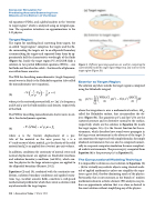
(Figure 5a). Inside the target region PC-ACOLOR finds a
((11))
TS((ff,,θ))=Liim20Log ⎜⎜
⎟⎟
rr→∞∞
solution to two partial differential equ0ati0ons (PDEs) – one
Figure 5. Different governing equati2ons are used for computing the −∇•(c∇u)−ω ρSu= fS
⎝⎝ 0 0 ⎠⎠
for fluids and the other for solids – that describe all phenom-
scattered field inside the target region (Figure 5a) and exterior to the target region (Figure 5b).
Exterior to Target Region:
The solution anywhere outside the target region is computed using the Helmholtz integral,
ena within linear acoustics.
The PDE for describing monochromatic (single frequency) sound waves in fluids is the Helmholtz equation (also called the monochromatic wave equation),
(2)
((22))
where the integration is over a mathematical surface, ∂ΩH, called the Helmholtz surface, that circumscribes the ob- jects (Figure 5b). The quantities p(r’) and ∂p(r’)/∂n are the scattered pressure and its derivative normal to the surface,
1100
rr p p
⎜⎜
⎟⎟
,=
r→∞
10⎜rp ⎟ ⎝00⎠
p = 0
⎜ω2ρ ⎟ B ⎝⎠
(4) and B and ρ are the bulk modulus and density, respectively,
where p is the scattered pressure field, ω= 2лf, f is frequency, of the fluid.
The PDE for describing monochromatic elastic waves in sol- ids is the elastodynamic equation,
(3)
where u is the (vector) displacement of a par- ticle of the material as the wave passes by, c is a 4th-rank tensor of elastic moduli, ρS is the density of the solid material and fS is an applied force (vector) per unit volume.
respectively, which are the solution to Equation (2) inside ((33))
In addition, conditions for continuity of normal stress and normal displacement are applied on fluid/solid interfaces
the target region. G(r, r’) is the Green’s function for the en- vironment, which describes how sound waves propagate in the large ocean environment in the absence of the target. It can sometimes be expressed with simple formulas for simple idealized environments but can also be computed numeri- cally in a separate computer simulation for more complicat- ed realistic environments. The pressure p(r) computed from Equation (4) is the pressure p(r) in Equation (1).
⌠⌠⎛⎛∂∂G((rr,,rrʹ′)ʹ′) ∂∂pp((rrʹ′)ʹ′)⎞⎞
and radiation boundary conditions (rad BCs), which con-
((44))
The Computational Modeling Technique
It is impossible to obtain an exact solution to Equations (2) – (4) for virtually any realistic objects using classical meth- ods of applied mathematics unless one simplifies the equa- tions a great deal, thereby eliminating much of the physics. Fortunately, that is not necessary, as the branch of modern mathematics known as finite-element (FE) analysis can pro- duce an approximate solution that is as close as desired to the exact solution without simplifying any of the physics.
pp((rr))= ⎜ pp((rrʹ′)ʹ′)−G((rr,,rrʹ′)ʹ′) ⎟ ddΓ ⎮⎮⎮⎮ ⎜ ∂∂nn ∂∂nn ⎟
tain the ph⌡y⌡s⌡ic⎝s⎝for the large exterior region, are ⎠a⎠pplied to ∂∂ΩΩ
the ellipsoidal boundary (Burnett, 2012).
HH
Equations (2) and (3), combined with the continuity con- ditions, radiation boundary conditions and applied excita- tions (e.g., incident acoustic field), constitute a well-posed mathematical problem for which there exists a solution valid anywhere inside the target region.
32 | Acoustics Today | Winter 2015
⎛⎛11 ⎞⎞ 11
−∇••⎜⎜ ∇pp⎟⎟ − pp = 00 ⎜⎜ 22 ⎟⎟
ωρ B ⎝⎝ ⎠⎠
⌠⌠⎛∂G(r,rʹ′) ∂p(rʹ′)⎞
p ( r ) = ⎮⌡ ⎮⌡ ⎜⎝ ∂ n p ( r ʹ′ ) − G ( r , r ʹ′ ) ∂ n ⎟⎠ d Γ
∂ΩH
−∇••((cc∇u))−ω ρ u= ff SS SS
22