Page 35 - \Winter 2015

FE analysis is an extension of classical calculus (Burnett, 1987). It began in the mid-20th century and has grown rap- idly, becoming such a powerful theoretical/numerical tech- nique that it can find solutions to virtually any differential or integral equations that model (simulate) applications of al- most any complexity. It has often been described as the most significant revolution in applied mathematics in the twenti- eth century, a perception that this author, who has worked with FE analysis for almost half a century, can heartily agree with. The merging of FE analysis with computer technology – two sciences that evolved concurrently and synergistical- ly – has created the modern discipline known as computa- tional mechanics (IACM, 2014). As computers continue to evolve, the power of FE analysis continues to grow apace. This article on predicting acoustic signatures is just one il- lustration of the power of modern computer simulation.
The essence of FE analysis is to subdivide the domain of a mathematical problem into a mesh of very small, sim- ply shaped “elements” and then to approximately repre- sent Equation (2) or (3) inside each and every element by transforming the differential equations into approximately equivalent algebraic equations. The algebraic equations in adjacent elements are interrelated, producing a continuity of physics across all the elements. Consequently, all of the ele- ment equations are coupled together into a very large system of simultaneous algebraic equations, typically hundreds of thousands or millions or even billions, which must then be solved on a computer. As elements in a mesh are made pro- gressively smaller, or the mathematical representation inside each element is enriched, the FE approximate solution be- comes progressively more accurate, converging eventually to the exact solution of the original mathematical problem.
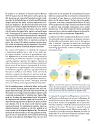
The FE modeling process is illustrated below for the prob- lem of acoustic scattering from a spherical steel shell rest- ing on (almost touching) a fluid-like sandy ocean bottom. In this model, the very large ocean and sediment regions can be considered mathematically as “infinitely large” regions (Fig- ure 6 (a)). To reduce the computational size of this problem, the large water and sediment regions can be replaced by a small surrounding ellipsoid (or spheroid or sphere) of water and sediment, with all the physics in the removed regions represented instead by mathematical relations, known as radiation boundary conditions, or rad BCs, applied to the outer boundary of the ellipsoid (Figure 6 (b)). This reduced model can be reduced further, to just one quadrant, by divid- ing it by any two perpendicular vertical planes intersecting the center of the spherical shell (Figure 6 (c)). One can then
analyze just the one quadrant by decomposing all acoustic fields into components that are symmetric or antisymmetric with respect to those planes, in a way that preserves all the physics in the reduced model. The last step in the model- ing process is to create a computationally efficient FE mesh for the quadrant model: larger elements away from the shell to represent long-wavelength propagating waves, smaller elements near to the shell to represent shorter-wavelength evanescent waves, and even smaller elements in the gap be- tween the shell and the ocean bottom (Figure 6(d)).
In addition to the above computational efficiencies, the mod- el is scaled with respect to frequency: as frequency increases, the ellipsoidal outer boundary moves closer to the targets in order to maintain a separation of about half a wavelength at all frequencies. This yields the additional advantage of maintaining approximately uniform modeling error across the frequency band.
Figure 6. (a) Full model: A spherical steel shell resting on the ocean bottom. The infinity symbols (∞) imply the water and sediment each
occupy an infinite “halfspace”. (b) Reduced model. (c) One quadrant of the reduced model. (d) The FE mesh for the quadrant model.
In summary, the computer modeling process consists of us- ing FE analysis to find numerical solutions to Equations (2) and (3) that describe the physics of wave propagation in flu- ids and solids, and then using Equation (4), in conjunction with those solutions, to find the scattered acoustic pressure anywhere in the ocean. This process is repeated over and over for different frequencies and different aspect angles. In- serting those scattered pressures into Equation (1) yields the sought-after TS as a function of frequency and aspect angle, which is the acoustic signature of the object.
| 33