Page 34 - 2017Spring

Speech Intelligibility Predictors
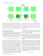
Figure 6. Example of a modulation filter bank. Each plot shows a spectrotemporal receptive field (STRF) for a different modula- tion filter, showing time-frequency regions of excitation (red) and regions of inhibition (blue). Filters with low temporal mod- ulation rates (close to the y-axis) prefer slower temporal fluctua- tions in the AN neurogram and filters with higher modulation rates prefer faster temporal oscillations. Filters with low spec-
Examples of Predictor
Computation Approaches
An example of how intelligibility can be predicted directly
from AN neurograms is the Neurogram SIMilarity (NSIM)
tral modulation scales (close to the x-axis) prefer broad spectral peaks and valleys in the AN neurogram and filters with high spectral modulation scales prefer more closely spaced spectral variations. Positive and negative temporal modulation rates correspond to downward and upward frequency sweeps, respec- tively, in the STRF. cyc/oct, Cycles/octave. Adapted from Bruce and Zilany (2007).
value is obtained by averaging the values computed for each 3×3 kernel, with a theoretical range of 0 (totally unintelligi- bility) to 1 (completely intelligible).
An important feature of the NSIM is that the time resolu-
tion of the AN neurogram can be adjusted such that it only
takes into account the mean-rate (MR) information in the
AN response (Figure 7, middle) or that it also includes fine-
timing (FT) information about neural spike times (Figure (1)
Alternative neurogram-based metrics include neural corre-
lation (Bondy et al., 2004; Christiansen et al., 2010), shuffled
metric developed by Hines and Harte (2012). A 3×3 time-
2 Equations_Bruce (Article 3) Please flush right in articles
frequency kernel is swept over the neurograms, and for each
of these kernels, an NSIM value is calculated according to
(1)
where the first term compares the “luminance” of the neuro-
gram images (i.e., the average intensity [μx] of each kernel),
the second term compares the visual “contrast” of the neuro-
αβγ ⎛2μμ+C⎞ ⎛2σσ+C⎞ ⎛σ+C⎞ NSIM(r,d)=⎜ 2 r r2 1 ⎟ ·⎜ 2 r d2 2 ⎟ ·⎜ rd 3 ⎟
7, bottom).
μ +μ +C σ +σ +C σσ +C ⎝rd1⎠⎝dd2⎠⎝rd3⎠
grams (i.e., the standard deviation [σx] in each kernel), and
2 Equations_Bruce (Article 3) Please flush right in articles correlation coupled with audio coherence (Kates and Are-
R−D2
the thSiTrdMIte=r1m− assesses the “structural” relationship between
hart, 2014), an orthogonal polynomial measure (Mamun et
R2
the two neurograms (conveyed as the Pearson product-mo-
(2)
ment correlation coefficient [σ ] in each kernel). The coef- xy
ficients α, β, and γ can take values between 0 and 1; for the speech material tested thus far in the literature, the optimal values for predicting speech intelligibility are α = γ ≈ 1 and β ≈ 0 (Hines and Harte, 2012; Bruce et al., 2013). The constants C1, C2, and C3 regularize the calculation in cases where the denominator may approach a value of 0. The overall NSIM
NSIM(r,d)=⎛ 2μrμr +C1 ⎞ ·⎛ 2σrσd +C2 ⎞ ·⎛ σrd +C3 ⎞ ⎜22⎟⎜22⎟⎜⎟
correlograms (Swaminathan and Heinz, 2012), envelope
al., 2015), and bispectrum analysis (Hossaiαn et al., 2016)β. γ
An example of a modulation-ba⎝se
temporal modulation index (STMI) developed by Elhilali et al. (2013), in which a normalized distance between the refer- ence and degraded spectrotemporal modulation spectra is computed according to
R−D2
STMI=1− R2 (2)
r
d
1
d
d
2
rd3⎠
d pr
edi
c⎠tor⎝ is
the
spe
c⎠ t r o⎝ -
μ +μ +C σ +σ +C σσ +C
32 | Acoustics Today | Spring 2017