Page 23 - WINTER2019

In triangulation, we invoke a powerful tool, the principal of reciprocity that states that sound propagation from a source to a listener is identical to the backpropagation from the lis- tener to the source. As such, the time it takes for an impulse of sound (a wave front) to reach a listener is equal to the time that it would take sound from the listener to propagate back to the origin. From this, we can form an isochron, which is a surface centered at the listener that connects points at which something occurs at the same time. Points on the isochron surface are all possible source origins. Thus, a single “listener” cannot determine exactly where the sound origin is located, being unable to distinguish where it lay exactly on its iso- chron. If a second listener saw and heard that event, likely with a different T based on its relative position to the source, its isochron and the intersection with the first identify the sound origin. Except when the listeners and source are in-line, the circular isochrons intersect at two points. A third listener reduces ambiguity.
Triangulation is the process of finding the precise location at the intersection of multiple isochrons. Now, if the listeners did not see the flash of lightning, then they do not know the T beforehand. A guess, or candidate event time, must be made from which to subtract the arrival time (when the thunder was heard), establishing a respective T to each listener. Figure 3 shows two examples of triangulation with three listeners based on two candidate event times. One candidate time is one-half of a second before the actual event time (Figure 3, top right); the three isochrons all intersect at different points surrounding the origin of sound. It is the third isochron that creates a solvable system of equations decoupled in range and time, such that all three isochron intersect only at one candidate event time. With the proper propagation speed, this equals the actual time (Figure 3, bottom right) and all three isochrons intersect at the sound origin. So, as a rule, three arrivals are needed to triangulate an unknown event.
Nuances of Hydroacoustic Triangulation
Sound speed in the ocean is not uniform in all directions, and although the free-space example was useful in thunderstorm ranging, it is far too simplistic to model ocean propagation. Sound speed is faster in warmer water and in deeper water due to hydrostatic pressure. Long-range acoustic propaga- tion in the ocean is possible due to trapping by upward and downward refraction (or reflection) processes. Consecutive surface reflections and refraction fold and distort a spheri- cally expanding wave front, elongating the duration of an impulse through a process called geometric dispersion. Geo-
metric dispersion of the San Juan signal, presumed to be an impulse with duration on the order of <1 second, caused an increase in the signal duration to well over 30 seconds.
To examine the dispersion and general signal timing (kine- matics), we can form acoustic rays, which are lines drawn normal to an expanding wave front. Rays represent the tra- jectory of sound traveling at the local speed of sound and integrating the reciprocal of sound speed along the ray gives the T to the ray terminus. Rays are defined by a launch angle (Ѳ), the starting angle of the ray trajectory. Asserting that a wave front spherically expands in the immediate vicinity of the source, meaningful rays can be launched upward, down- ward, or horizontal. The largest ±Ѳ that avoids a surface (and/ or bottom) reflection is the limiting ray.
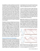
Figure 4 shows a group of rays, or ray fan, spanning the lim- iting ray for two environments that are representative of the ocean structure encountered by the propagating San Juan signal. Figure 4, left top, shows a polar environment idealized as a 17 m/s increase in sound speed per kilometer of depth; Figure 4, left bottom, is representative of a midlatitude ocean, which, in addition to the increase in sound speed with depth, has a warm layer in the upper ocean and thus has a higher speed near the surface and a minimum close to 1,000 meters deep. The rays in these two environments follow different
Figure 4. Left: depth-dependent sound speed profile for a polar profile (top) and a midlatitude profile (bottom). Right: acoustic ray fans for the two environments spanning the limiting angle: red lines, rays launched upward; black lines, rays launched downward.
Winter 2019 | Acoustics Today | 23